Mathematical Methods

Use this volume as a task router, not as a mathematics course that must be completed before QFT. Start by identifying the mathematical object or manipulation in the calculation—linear map, limit, contour, distribution, differential operator, spectrum, bundle, constraint, probability law, or asymptotic regime. Enter at the first missing capability, follow only the prerequisites used by the argument, and continue to the relevant physics or theorem-level treatment once the reusable mathematics is established.

There is no volume-wide hard or recommended prerequisite. The practical non-gating floor is multivariable calculus, elementary matrices, ordinary differential equations, basic quantum mechanics, and special relativity. Even that preparation should be checked capability by capability: difficulty with topology does not block Fourier methods, uncertainty about stochastic calculus does not block spinors, and the advanced categorical chapter does not gate any earlier chapter.

The volume supplies hypothesis-aware algebra, analysis, convex certification, geometry, topology, variational methods, probability, asymptotics, and bounded bridges to advanced language. It develops definitions, legal transformations, counterexamples, convention translations, and small QFT-facing examples. Developed dynamics, phenomenology, renormalization prescriptions, physical state selection, production software, and theorem-first mathematical QFT continue in the destinations linked below.

The thirteen chapter groups appear in a stable reference order. That order is not a prerequisite ladder. Across the 87 topic pages there are seventeen zero-hard-prerequisite entrances, and no valid route requires reading all thirteen chapters.

Diagnose · Choose a route · Dependency map · Conventions · Chapter guide · Threads · Scalar kernel · Monopole · Certificate · Review · Continue

Diagnose the missing capability

The overview itself has no prerequisite. Use each row independently and repair only the gap that affects the route you need.

Observable readiness checks and the shortest local repair

Check	Ready evidence	If unsure	Repair and re-entry
Can you type vectors, covectors, linear maps, adjoints, tensor factors, and graded signs without relying on an accidental basis identification?	Write the domain and codomain of every map and distinguish a dual pairing from an inner product.	Test one basis change and one Grassmann sign by returning to the invariant map.	Use Linear and tensor methods repair, then enter Linear, Tensor, and Graded Algebra.
Can you name the theorem that licenses a limit, sum, integral, Fourier transform, or change of variables?	State the measure, convergence mode, dominating or integrability hypothesis, and transform normalization.	Try to construct a counterexample after removing one hypothesis.	Enter Analysis, Measure, and Fourier Methods; for the kernel route, use Fourier, distributions, and Green functions repair.
Can you move a contour while tracking orientation, endpoints, branches, sheets, singularities, and decay at infinity?	Draw the original and deformed cycles and list every crossed or avoided obstruction.	Distinguish an algebraic substitution from a legal deformation.	Use Complex and asymptotic methods repair, then enter Complex Analysis and Analytic Continuation.
Can you state what a singular kernel acts on and specify an operator together with its spaces, domain, data, and intended inverse?	Write the test-function pairing and verify the Green equation and support or boundary condition.	Check whether a pointwise product, pullback, or inverse is actually defined.	Combine Distributions and Microlocal Methods, Differential Equations and Green Operators, and, when domains matter, Functional and Spectral Analysis.
Can you distinguish a group, Lie algebra, representation, field label, particle representation, local frame, and global bundle?	Translate a transformation through one overlap map or intertwiner and recover an invariant quantity.	Separate gauge-bundle data from spacetime-frame data before comparing connections.	Use Relativity, Lorentz symmetry, and spin repair, then choose Groups and Spinors, Geometry and Bundles, or Topology and Characteristic Classes.
Can you vary an action while preserving boundary terms and identifying degenerate directions separately from physical variations?	Derive the bulk Euler–Lagrange term, boundary contribution, and presymplectic kernel independently.	Test whether an imposed boundary condition or quotient was used silently.	Use Variational and classical-field repair, then enter Variational, Symplectic, and Constraint Methods.
Can you distinguish a probability measure, a law, a density, a random distribution, a stochastic process, and a formal path-integral weight?	Name the probability space or regulated measure and state the hypotheses of every limit theorem.	Check whether covariance determines the law, whether detailed balance was assumed, and whether correlations are summable.	Use Statistical ensembles and probability repair, then enter Probability and Stochastic Processes.
Can you state an approximation with its limit, fixed data, sector, uniform set, branch, truncation order, and remainder?	Give a fixed-order error statement and identify the first point where it becomes nonuniform.	Separate convergence, asymptoticity, optimal truncation, and special-function boundary selection.	Use Complex and asymptotic methods repair, then enter Asymptotic and Special-Function Methods.
Can you type objects, morphisms, variance, weak equivalences, monoidal data, and local-to-global maps in a modern QFT source?	Check every composite and say which stronger theorem the source actually invokes.	Begin with the smallest category or chain-complex example rather than importing the vocabulary wholesale.	Enter the optional Categorical, Homological, and Local-to-Global Language bridge, then continue to Mathematical QFT for specialist theorems.

The mathematical readiness diagnostic checks linear/tensor, Fourier/distribution/Green-operator, and complex/asymptotic capabilities independently. The classical-field and relativity diagnostic and statistical/probability diagnostic cover different capability sets. The chapter overviews provide more specialized checks.

For a structured study sequence rather than a local repair, use Mathematical Foundations for Physicists. It organizes preparation; it is not a completion claim for this volume.

Choose the shortest route

An arrow in the table means “continue through this capability when the target argument uses it,” not “read the entire chapter.” A slash marks a genuine choice between branches. The last column states where the developed physical question continues.

Reader-intent routes through Mathematical Methods

QFT need	Minimum mathematical route	Observable exit and stopping point
Core free fields	Selected Linear Algebra → Fourier Methods or Complex Analysis → Distributions → Differential Equations → Field Variations.	Construct a regulated kernel with its equation, contour or support data, and source normalization; continue to Foundations for states, quantization, and physical propagators.
Symmetry and gauge theory	Linear Algebra → Groups and Representations → Geometry and Bundles → selected Topology.	Translate local connection data into curvature, holonomy, and characteristic information; continue to Symmetry and Gauge Structure for gauge physics and anomalies.
Rigorous QFT preparation	Analysis and Measure → Distributions → Functional Analysis → selected Categorical Language.	State spaces, domains, singular products, topologies, and typed maps precisely; continue to Mathematical QFT for theorem-first frameworks.
Certified conformal bootstrap	Selected Linear Algebra → Convex Cones, Separation, Conic Duality, and Semidefinite Programs.	Formulate a finite conic feasibility problem and state exactly what an exact separating certificate proves; continue to Conformal Field Theory and Bootstrap for crossing physics and to computational workflows for verified execution.
Stochastic or lattice work	Analysis and Measure → Probability and Stochastic Processes.	State the law, stochastic convention, limit-theorem hypotheses, and autocorrelation-aware uncertainty; continue to Thermal and Nonequilibrium QFT or Lattice and Hamiltonian QFT.
Semiclassical methods	Complex Analysis or Differential Equations → Variational Methods → Asymptotic Methods.	Identify stationary structures, legal cycles, fluctuation operators, branches, and remainders; continue to Nonperturbative Dynamics for physical saddle sectors and tunneling.
Curved-spacetime modes	Geometry → Differential Equations → Distributions → Functional Analysis → Special Functions.	Select and normalize modes with geometry, domain, boundary, and state data visible; continue to QFT in Curved Spacetime for states, particles, and renormalized observables.

Reference order is not prerequisite order

The volume contains 87 topic pages, 102 direct hard-prerequisite links, and 36 recommended-preparation links. The longest hard chain has depth five. Those numbers describe a sparse page-level graph: they do not turn a chapter title into a blanket prerequisite. Every chapter overview has no hard prerequisite, and seventeen topic pages can be entered without one.

The table below compresses cross-chapter hard links between individual topic pages. A row means that at least one page in the target chapter uses preparation from the source chapter. It does not mean that every page in the target requires the whole source chapter.

Compressed cross-chapter hard-prerequisite connections

Preparation source	Target chapters containing at least one dependent page	What the connection supplies
Linear, Tensor, and Graded Algebra	Functional/Spectral Analysis; Groups/Representations/Spinors; Probability; Variational/Constraint Methods.	Typed maps, duality, forms, finite spectra, and invariant signs.
Analysis, Measure, and Fourier Methods	Differential Equations; Probability; Asymptotic/Special-Function Methods.	Measures, Lebesgue integration, function spaces, and convergence hypotheses.
Complex Analysis and Analytic Continuation	Asymptotic and Special-Function Methods.	Holomorphic and Cauchy theory used by the Mellin-analysis branch.
Distributions and Microlocal Methods	Differential Equations; Functional/Spectral Analysis.	Test functions, distributions, support, and the meaning of singular kernels.
Differential Equations and Green Operators	Asymptotic and Special-Function Methods.	ODE evolution, boundary data, elliptic heat kernels, and operator equations.
Functional and Spectral Analysis	Topology/Characteristic Classes; Asymptotic/Special-Function Methods.	Fredholm structure, spectra, resolvents, and functional calculus.
Lie Groups, Representations, and Spinors	Differential Geometry/Bundles; Variational/Constraint Methods.	Group actions, Lie algebras, representations, and Clifford/Spin-group algebra.
Differential Geometry and Bundles	Topology, Cohomology, and Characteristic Classes.	Manifolds, forms, bundles, connections, curvature, and orientation.
Topology, Cohomology, and Characteristic Classes	Categorical, Homological, and Local-to-Global Language.	Chains, cochains, homology, and exact sequences for one advanced branch.
Variational, Symplectic, and Constraint Methods	Asymptotic and Special-Function Methods.	Symplectic geometry and generating data for semiclassical phases.

Recommended preparation is deliberately weaker: it improves fluency but does not block the target argument. Likewise, a first-application or developed-treatment link points outward; it never creates a prerequisite in the opposite direction.

State the complete problem before calculating

The site’s global conventions apply throughout the volume. Lorentzian examples use signature $(+---)$ in four dimensions and $(+,-,\ldots,-)$ in $d$ dimensions; $\hbar=c=k_{\mathrm B}=1$; differentials are roman; inner products are conjugate-linear in the bra and linear in the ket; and Lie-algebra generators are Hermitian unless a page translates another convention explicitly.

The default Fourier pair is

$$\widetilde f(p) = \int \mathrm d^d x\, e^{+ip\cdot x}f(x), \qquad f(x) = \int\frac{\mathrm d^d p}{(2\pi)^d}\, e^{-ip\cdot x}\widetilde f(p),$$

so $\partial_\mu\mapsto-ip_\mu$. Every page that imports another phase or normalization translates it locally.

Before manipulating an expression, record the data appropriate to its type:

• Algebra: scalar field, vector spaces, domains and codomains, dual pairings, forms, grading, and basis dependence.
• Limits and integrals: measure, convergence mode, integrability or domination, order of limits, and exceptional parameter values.
• Complex analysis: branch, cut, base point, sheet, continuation path, contour orientation, endpoints, large-arc behavior, and $i0$ boundary value.
• Distributions and operators: test-function space, singular support or wavefront condition when relevant, operator spaces and domain, boundary/initial/support data, and zero-mode rule.
• Symmetry and geometry: global group, representation, manifold dimension and signature, orientation, bundle, local trivializations, connection convention, and curvature sign.
• Variational systems: allowed variations, boundary conditions, bulk and boundary terms, constraint surface, quotient, and presymplectic kernel.
• Probability and stochastic dynamics: probability space or regulated measure, law, reference measure for a density, Itô or Stratonovich convention, generator domain, and hypotheses of every limit theorem.
• Asymptotics: limiting direction, fixed data, sector, branch, uniform parameter set and norm, truncation order, and remainder meaning.
• Categorical language: objects, typed morphisms, variance, chosen weak equivalences, monoidal data, and the exact local-to-global condition.
• Numerical evidence: finite problem, scaling, tolerances, residuals, conditioning, precision, and the analytic statement independently checked.

Convention translation ends with an invariant check. Useful checks include a round trip under change of basis, a Fourier inversion, a contour reconstructed from its boundary values, a Green equation, preservation of a Wronskian or spectrum, a flux integer, equality of two index formulas, normalization of a probability law, or a primal–dual residual identity. Agreement of symbols without one such check is not enough.

The analysis and distributional hypotheses behind these checks are developed in Axler 2020, §§2B–3B, 5A–5B, 7A–7B, and 11A–11C, pp. 25–99, 117–135, 194–208, and 340–377, Open PDF and Dyatlov 2022, §§5.1–5.2, 7.2, 9.1, and 11.1–11.3, official lecture-note PDF. For operator domains, resolvents, and the self-adjoint spectral theorem, see Teschl 2014, §§2.4, 3.1, and 3.4, Open PDF.

Exact chapter guide

Linear, Tensor, and Graded Algebra

Open the chapter overview. Its six pages build the finite-dimensional invariant and graded algebra used for fields, states, symmetries, and fermionic variables. Enter through Vector Spaces for typed maps and duals, or through the tensor branch when the immediate issue is grading, Grassmann variables, and Berezin integration.

The observable result is an invariant formulation with adjoints, projectors, tensor symmetries, or graded signs checked under a basis change. Finite spectral theorems, Jordan forms, and matrix adjoints do not settle infinite-dimensional domains, self-adjointness, or spectral measures; those continue in Functional and Spectral Analysis.

Analysis, Measure, and Fourier Methods

Open the chapter overview. Its seven pages have three independent entrances: limits and completeness, measures and integration, and Fourier theory. The chapter supplies the convergence, integration, function-space, convolution, and transform tools that formal QFT manipulations often leave implicit.

The observable result is a named theorem with its hypotheses, or a Fourier calculation with normalization and function-space meaning visible. A basic transform calculation does not require the entire measure branch; theorem- level interchange and $L^p$ claims do require their stated preparation.

Complex Analysis and Analytic Continuation

Open the chapter overview. Its five pages begin with Cauchy theory and branch into residues, branches and sheets, boundary values, and legal contour deformation. Enter through the operation in front of you rather than treating analytic continuation as a single mnemonic.

The observable result is a contour or boundary-value statement with orientation, cuts, singularities, endpoints, and growth conditions recorded. Amplitude domains, unitarity, positivity, physical dispersion relations, and state interpretation continue in Scattering or Foundations.

Distributions and Microlocal Methods

Open the chapter overview. Its six pages replace singular-function shorthand by pairings on test-function spaces. Delta calculus, tempered Fourier methods, distributional kernels, extension problems, and the wavefront bridge branch from that foundation rather than forming one chain.

The observable result is a singular operation with its test space and legal product, pullback, or support condition stated. The bounded microlocal pages do not prove propagation-of-singularities theorems, construct Hadamard states, or develop Epstein–Glaser renormalization; those continue in Mathematical QFT, Curved Spacetime, or Renormalization.

Differential Equations and Green Operators

Open the chapter overview. Its seven pages connect ODE evolution, symbols and PDE type, weak solutions, well-posedness, fundamental solutions, causal propagators, elliptic boundary problems, and heat kernels. Linear ODEs and principal symbols are independent entrances; Green-operator pages add spaces and data before an inverse is written.

The observable result is an equation together with its operator domain, initial or boundary conditions, support prescription, and verification identity. A principal symbol classifies leading behavior but does not select an inverse or prove well-posedness. Physical propagator meaning and global curved-spacetime theory continue elsewhere.

Functional and Spectral Analysis

Open the chapter overview. Its nine pages contain two genuinely different entrances. The finite-dimensional convex branch develops cones, separation, conic duality, semidefinite programs, and certificate logic. The infinite-dimensional branch develops Banach and Hilbert spaces, bounded and unbounded operators, self-adjoint extensions, spectra, resolvents, trace ideals, and bounded bridges to operator algebras and nuclear spaces.

The observable result is either an exact finite-dimensional certificate with its qualification, or an operator statement whose topology and domain are part of the claim. Symmetric does not mean self-adjoint, and a small floating-point residual is not an exact feasibility certificate. The finite-dimensional duality framework is developed in Boyd and Vandenberghe 2004, Chapters 2, 4, and 5, author-hosted PDF.

Lie Groups, Representations, and Spinors

Open the chapter overview. Its seven pages distinguish groups, covers, Lie algebras, representations, intertwiners, roots and weights, Lorentz and Poincaré representations, Clifford algebras, Spin groups, and spinors. Elementary groups, spacetime representations, and Clifford/spinor methods are separate entrances.

The observable result is a symmetry statement with global group form, generator convention, representation space, conjugation, chirality, and signature visible. A Lorentz field representation is not a unitary Poincaré particle representation, and Clifford theory does not require the Lorentz page. See Hall 2015, Chapters 1–5 and 7–13, publisher record for the group and representation structure.

Differential Geometry and Bundles

Open the chapter overview. Its eight pages begin from manifolds and branch to forms, metric geometry, bundles, connections, holonomy, spin structures, and Dirac operators. Gauge-bundle connections and spacetime Levi–Civita or spin connections share geometric language but are different objects.

The observable result is a coordinate or patch calculation translated into a global tensor, form, bundle, connection, curvature, or holonomy statement. Local representatives do not by themselves prove that a global bundle, connection, or spin lift exists. Developed gauge and gravitational physics continues in their corresponding volumes.

Topology, Cohomology, and Characteristic Classes

Open the chapter overview. Its six pages have independent entries through homotopy and winding, chains and cohomology, and bordism. Differential forms join the de Rham branch; bundle connections join characteristic classes; spectra and spin geometry join the index bridge.

The observable result names the equivalence relation detected by an invariant and fixes coefficients, orientation, and normalization. An index counts kernel minus cokernel under Fredholm hypotheses; it is not by itself an anomaly calculation. Characteristic numbers and bordism data do not automatically classify QFT phases. Geometry and topology conventions used in these chapters are developed in Nakahara 2003, Chapters 3–7 and 9–10 and §§11.1–11.6, 12.1–12.2, and 12.6, publisher record.

Variational, Symplectic, and Constraint Methods

Open the chapter overview. Its six pages begin independently with field variation or symplectic geometry, then develop second variation, moment maps, constraints, reduction, presymplectic degeneracy, and covariant phase-space ambiguities.

The observable result keeps bulk equations, boundary terms, constraint surfaces, quotient directions, and degeneracies distinct. Symplectic forms are alternating forms, not inner products; restricting to a constraint surface and quotienting its null directions are different operations. See Cannas da Silva 2006, Lectures 1, 2, 8, and 18 and §§22.1, 22.4, 24.1, and 26.1–26.4, Open PDF.

Probability and Stochastic Processes

Open the chapter overview. Its seven pages begin after measure and Lebesgue integration, then branch to limit theorems, generating objects and Gaussian structure, or general stochastic processes. Brownian/Langevin dynamics follows process foundations, while Markov sampling error also joins the limit-theorem branch.

The observable result distinguishes measures, laws, densities, random distributions, stochastic trajectories, generators, semigroups, and uncertainty estimates. Stationarity is not ergodicity, invariance is not reversibility, and Markov dynamics need not be self-adjoint. These distinctions are developed in Pavliotis 2014, §§1.1–1.3, 2.2–2.4, 3.1–3.5, 4.1, and 4.6, pp. 1–13, 30–39, 49–66, 77–80, and 104–105, Open PDF.

Asymptotic and Special-Function Methods

Open the chapter overview. Its eight pages include several independent routes. Asymptotic scales lead to Laplace, stationary-phase, and WKB branches; Mellin analysis enters from integration and Cauchy theory; exact special functions enter directly from linear ODEs; heat/zeta methods join Mellin, elliptic, and spectral inputs.

The observable result states the limit, sector, uniformity, branch, boundary data, and remainder. An asymptotic series need not converge, a saddle need not lie on an accessible cycle, and a special-function name does not select a physical mode. Heat/zeta methods here stop before selecting a physical one-loop determinant or renormalization scheme; continue to Renormalization and Effective Field Theory, Nonperturbative Dynamics, or QFT in Curved Spacetime as the problem requires. Full resurgence and physical saddle sectors likewise continue in Nonperturbative Dynamics. Riemann-surface and modular physics continue in Conformal Field Theory and Bootstrap. Hunter develops these distinctions in Hunter 2004, Chapter 2 and §§3.1 and 3.3–3.6, pp. 19–47, Open PDF; canonical formulas and sector data are maintained in NIST DLMF 2026, Chapters 2, 9, 10, 15, and 25.

Categorical, Homological, and Local-to-Global Language

Open the chapter overview. This five-page advanced bridge begins with categories and functors, then branches in parallel to monoidal language, chain homotopy and quasi-isomorphisms, or sheaf/cosheaf and local-to-global language. The homological branch also uses the earlier chains-and-cochains page; all three branches meet only at the final framework boundary.

The observable result is accurate vocabulary with objects, maps, weak equivalences, monoidal data, and descent conditions typed. It does not construct higher categories, prove Weiss descent, or develop derived or factorization QFT. Continue to Mathematical QFT for those frameworks. The foundational categorical definitions are presented in Leinster 2014, Introduction and Chapter 1, §§1.1–1.3, pp. 1–40, arXiv record.

Six recurring threads

The same examples recur so that a reader can see what each mathematical viewpoint adds. These are application routes, not declarations that every stage is a hard prerequisite.

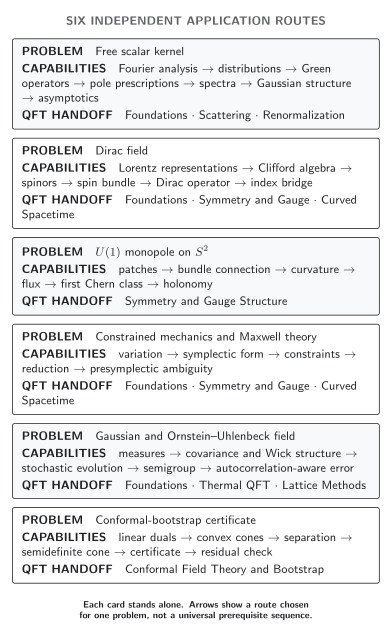
Read the figure from left to right along the row that matches the problem in front of you. The absence of vertical arrows is essential: no row requires a reader to complete the rows above it.

Each row gives one application-driven route from a recurring problem to later QFT work. Arrows mean continuation within that row, not a universal prerequisite relation. The map is qualitative, schematic, and not to scale; the table below supplies the complete route, check, and handoff in text.

Six cross-chapter examples and their developed continuations

Thread	Mathematical route	Invariant check and continuation
Free scalar kernel	Fourier analysis → distributions → PDE and Green operators → pole prescriptions → spectra → Gaussian structure → asymptotics.	Verify the Green equation, boundary value, covariance positivity only in the regulated Euclidean setting, and asymptotic regime. Continue to Foundations, Perturbative QFT and Scattering, or Renormalization and Effective Field Theory.
Dirac field	Lorentz representations → Clifford algebra → spinors → spin bundle → Dirac operator → index bridge.	Check the Clifford relation, spin lift, operator domain, signature translation, and index grading. Continue to Foundations, Symmetry and Gauge Structure, or Curved Spacetime.
U(1) monopole on the two-sphere	Patches → bundle connection → curvature → flux → characteristic class → holonomy.	Check that transition winding, normalized flux, and first Chern number agree under one orientation and gauge convention, and that loop holonomy is unchanged by a compatible change of local trivialization. Continue to Symmetry and Gauge Structure.
Constrained mechanics and Maxwell	Variation → symplectic form → constraints → reduction → presymplectic ambiguity, with algebra and Lie symmetry added where required.	Preserve the boundary term and distinguish restriction, quotient, and null directions. Continue to Foundations, Symmetry and Gauge Structure, or Curved Spacetime.
Gaussian and Ornstein–Uhlenbeck field	Covariance → Wick structure → stochastic evolution → semigroup → autocorrelation-aware error, after measure and integration preparation.	Check probability normalization, covariance, generator/forward duality, and observable-specific sampling variance. Continue to Foundations, Thermal/Nonequilibrium QFT, or Lattice Methods.
Conformal-bootstrap certificate	Linear duals → convex and dual cones → separation → primal–dual conic form → positive-semidefinite cone → certificate and residual check.	Verify exact dual feasibility and a strict separating sign; keep numerical residuals separate. Continue to Conformal Field Theory and Bootstrap.

The free scalar kernel across the volume

This thread shows why a formula for a denominator is not yet a propagator. Begin in Euclidean $\mathbb R^d$ with $m>0$ and

$$A_E=-\partial_E^2+m^2, \qquad D(A_E)=H^2(\mathbb R^d) \subset L^2(\mathbb R^d).$$

Write $p_E\cdot x_E=\sum_{a=1}^d p_E^a x_E^a$ and $p_E^2=p_E\cdot p_E$ for the positive-definite Euclidean pairing. With the volume’s Fourier convention, $A_E$ is multiplication by $p_E^2+m^2$, so its inverse kernel is the tempered distribution

$$G_E(x_E) = \int\frac{\mathrm d^d p_E}{(2\pi)^d}\, \frac{e^{-ip_E\cdot x_E}}{p_E^2+m^2}, \qquad A_EG_E=\delta^{(d)}(x_E).$$

Fourier analysis diagonalizes translation invariance. Distribution theory states what the singular kernel acts on. Green-operator theory adds the operator domain and verifies the source normalization. Spectral calculus recognizes $A_E^{-1}$ as a bounded function of this positive self-adjoint realization.

The elementary Schwinger identity,

$$\frac{1}{p_E^2+m^2} = \int_0^\infty e^{-t(p_E^2+m^2)} \,\mathrm dt,$$

gives the exact heat representation

$$G_E(x_E) = \int_0^\infty \frac{\mathrm dt}{(4\pi t)^{d/2}}\, \exp\left( -m^2t-\frac{|x_E|^2}{4t} \right).$$

For $d=4$ and $r=|x_E|>0$,

$$G_E(r) = \frac{m}{4\pi^2r}K_1(mr).$$

The integral representation and large-argument expansion are NIST DLMF 2026, §10.32(i), Equation 10.32.10 and NIST DLMF 2026, §10.40(i), Equation 10.40.2. They give, as $mr\to+\infty$ on the positive real axis,

$$\begin{aligned} G_E(r) &= \frac{\sqrt m} {4\sqrt2\,\pi^{3/2}r^{3/2}} e^{-mr}\\ &\quad\times \left[ 1+\frac{3}{8mr} +\mathcal O\!\left((mr)^{-2}\right) \right]. \end{aligned}$$

This asymptotic statement is not uniform at $r=0$ and says nothing about a truncation order growing with $mr$.

In a finite-dimensional Euclidean regulator—for example, a finite lattice with finitely many sites or an explicit finite-mode cutoff—a positive-definite matrix $A_E$ defines a genuine normalized Gaussian calculation. Finite spatial volume alone is not an ultraviolet regulator. For

$$S_E[\phi;J] = \frac12\langle\phi,A_E\phi\rangle -\langle J,\phi\rangle,$$

completion of the square gives

$$\frac{Z_E[J]}{Z_E[0]} = \exp\left[ \frac12 \langle J,A_E^{-1}J\rangle \right].$$

The inverse is the covariance and source derivatives generate Wick pairings. This finite-dimensional identity does not by itself construct a continuum Gaussian measure or define local products of a random distribution.

In Lorentzian signature $(+---)$, a physical boundary-value choice is extra data. With $p\cdot x=p^0x^0-\mathbf p\cdot\mathbf x$,

$$\Delta_F(x) = \int\frac{\mathrm d^4p}{(2\pi)^4}\, \frac{i\,e^{-ip\cdot x}} {p^2-m^2+i0},$$

and

$$(\Box+m^2)\Delta_F(x) = -i\delta^{(4)}(x).$$

The distributional identity

$$\frac{1}{u+i0} = \operatorname{PV}\frac1u -i\pi\delta(u)$$

fixes the boundary value. It is not disposable notation and cannot be recovered from the algebraic denominator alone. Retarded, advanced, Feynman, and Euclidean kernels solve related operator equations with different support, boundary, or analytic data. The distributional Fourier calculus is treated in Dyatlov 2022, §5.2.3 and Exercise 5.4(c), pp. 63–65, and §§11.1–11.2, pp. 119–134, official lecture-note PDF; the stated $(+---)$ Feynman convention and Klein–Gordon normalization are checked in Tong 2006, §2.7, Equations 2.174–2.175.

The complete thread therefore preserves seven distinct questions:

1. Which transform diagonalizes the equation?
2. In which distribution space does the multiplier act?
3. Which operator realization and data select an inverse?
4. Which contour or boundary value selects the Lorentzian kernel?
5. Which spectral representation reorganizes the same realization?
6. When does a regulated positive inverse define Gaussian covariance?
7. In which limit and region does an asymptotic form approximate the exact kernel?

No one answer substitutes for the others.

One integer from patches, curvature, and index

The Dirac and monopole threads meet in a controlled Riemannian example. First keep the Lorentzian algebraic stage distinct. In the site’s $(+---)$ convention,

$$\{\gamma^\mu,\gamma^\nu\} = 2\eta^{\mu\nu}\mathbf1, \qquad p\!\!\!/ \equiv \gamma^\mu p_\mu, \qquad (p\!\!\!/)^2=p^2\mathbf1.$$

The Riemannian index problem uses a translated convention. Take Euclidean gamma matrices with

$$\{\gamma_E^a,\gamma_E^b\} = 2\delta^{ab}\mathbf1, \qquad c(e^a)=i\gamma_E^a, \qquad c(\xi)^2=-|\xi|^2\mathbf1.$$

A Clifford module is local algebraic data. A spin structure is a principal Spin bundle equipped with a two-fold equivariant map to the oriented orthonormal frame bundle. After choosing a Spin representation $\rho$, the spinor bundle, spin connection, and Dirac operator fit into

$$\begin{gathered} P_{\mathrm{Spin}} \xrightarrow{\lambda} P_{\mathrm{SO}} \longrightarrow M, \qquad S=P_{\mathrm{Spin}}\times_\rho\Sigma,\\ \nabla^S \longrightarrow \mathcal D=c\circ\nabla^S. \end{gathered}$$

The operator also requires a specified domain. This spin-lift and Dirac construction is developed in Nakahara 2003, §11.6, publisher record.

Now orient $S^2$ by $\sin\theta\,\mathrm d\theta\wedge\mathrm d\varphi$, cover it by northern and southern patches, and take the Hermitian line bundle $L_n\to S^2$ with

$$g_{NS}(e^{i\varphi}) = e^{in\varphi}, \qquad n\in\mathbb Z.$$

In the coupling-absorbed real connection convention, choose the global curvature

$$f = \frac n2\sin\theta\, \mathrm d\theta\wedge\mathrm d\varphi.$$

With the equator oriented by increasing $\varphi$ and $v_N=g_{NS}v_S$,

$$\begin{aligned} \frac{1}{2\pi i} \int_{S^1} g_{NS}^{-1}\,\mathrm dg_{NS} &= \left\langle c_1(L_n),[S^2]\right\rangle\\ &= \frac1{2\pi}\int_{S^2}f = n. \end{aligned}$$

Equip the sphere with its Riemannian metric and spin structure and $L_n$ with a compatible unitary connection. On the compact sphere, use the standard Sobolev realization and the chirality grading $S=S^+\oplus S^-$. With the index chapter’s convention, the twisted chiral operator

$$\mathcal D_{R,L_n}^+ : H^1(S^2;S^+\otimes L_n) \longrightarrow L^2(S^2;S^-\otimes L_n)$$

is Fredholm and satisfies

$$\operatorname{ind} \mathcal D_{R,L_n}^{+} = n.$$

The equality compares transition winding, a de Rham period, an integral first Chern number, and a Fredholm index. It depends on orientation, transition direction, curvature normalization, Riemannian signature, unitary connection, ellipticity, compactness, and grading. Reversing one convention changes the corresponding signs coherently; it must not be repaired by changing only the last formula. The patch, flux, characteristic-class, and index calculations are supported by Nakahara 2003, §10.5.2, Example 11.2, and §12.6, pp. 400–401, 432–433, and 468–472, publisher record.

This mathematical equality is not an anomaly coefficient, a classification of gauge sectors, or a proof that a monopole solution is dynamically realized. Those physical questions continue in Symmetry and Gauge Structure and the gauge-theory volumes.

A finite certificate and its claim ceiling

Let $V$ and $W$ be finite-dimensional real vector spaces, let $K\subseteq V$ be a closed convex cone, let $A:V\to W$ be linear, and consider

$$Ax=b, \qquad x\in K.$$

The dual cone and algebraic adjoint are

$$\begin{aligned} K^* &= \{\ell\in V^*:\langle\ell,x\rangle\ge0 \text{ for every }x\in K\},\\ A^* &: W^*\longrightarrow V^*, \qquad \langle A^*q,x\rangle=\langle q,Ax\rangle. \end{aligned}$$

The attainable right-hand sides form $A(K)$. Strong separation gives the always-valid alternative

$$\begin{gathered} b\in\overline{A(K)},\\ \text{or there is }q\in W^* \text{ such that } A^*q\in K^*, \quad \langle q,b\rangle<0. \end{gathered}$$

The two lines cannot both hold because, for $x\in K$,

$$\langle q,Ax\rangle = \langle A^*q,x\rangle \ge0.$$

When $A(K)$ is closed, the second line is an exact infeasibility certificate. For semidefinite cones, however, a linear image can fail to be closed. A problem can then be infeasible but arbitrarily close to feasible, with no certificate of this elementary strict-separation form. Strong duality and attainment are separate properties. An appropriate relative-interior Slater condition is sufficient, not necessary: with feasibility and a finite optimum, strict feasibility on one side gives zero gap and attainment on the opposite side, while suitable qualifications on both sides give attainment of both optima. Weak duality alone supplies none of those conclusions. These distinctions are developed in Boyd and Vandenberghe 2004, Chapters 2, 4, and 5, author-hosted PDF and the semidefinite pathologies in Liu and Pataki 2015, §§1–3, pp. 1441–1454.

A finite conformal-bootstrap truncation turns normalized crossing data and positivity assumptions into a cone or semidefinite feasibility question. An exact separating functional can exclude that finite problem. A numerical candidate becomes an exact result only after coefficients, positivity, and residual signs are independently bounded. Failure to find a certificate does not prove that a CFT exists, and a certificate for a finite approximation does not automatically establish the infinite-dimensional claim. The finite-functional cone construction is developed in Rattazzi, Rychkov, Tonni, and Vichi 2008, §§4–5.2.

One Ornstein–Uhlenbeck mode from law to error bar

Let $\gamma,D>0$ and use the Itô convention

$$\mathrm dX_t = -\gamma X_t\,\mathrm dt +\sqrt{2D}\,\mathrm dW_t.$$

The invariant law is $N(0,D/\gamma)$. In stationarity,

$$C(\tau) = \operatorname{Cov}(X_0,X_\tau) = \frac{D}{\gamma} e^{-\gamma|\tau|},$$

and the backward generator on a suitable test-function domain is

$$Lf(x) = -\gamma x f'(x)+D f''(x).$$

The semigroup acts on observables, while its adjoint evolves laws. Invariance does not imply reversibility in general, although this one-dimensional gradient example is reversible with respect to its Gaussian invariant law.

For the continuous time average

$$\overline X_T = \frac1T\int_0^T X_t\,\mathrm dt,$$

Gaussianity and the exact covariance give

$$\begin{aligned} \operatorname{Var}(\overline X_T) &= \frac{2}{T^2} \int_0^T (T-\tau)C(\tau)\,\mathrm d\tau\\ &= \frac{2D}{\gamma^2T} - \frac{2D(1-e^{-\gamma T})} {\gamma^3T^2}. \end{aligned}$$

Thus the leading long-time variance is $2D/(\gamma^2T)$, with an explicit finite-$T$ correction. This conclusion is observable-specific; a nonlinear observable has a different correlation function and effective uncertainty. The process, generator, forward equation, invariant law, and reversibility distinctions are developed in Pavliotis 2014, §§1.1–1.3, 2.2–2.4, 3.1–3.5, 4.1–4.2, 4.4, and 4.6, Equations 4.18–4.24 and 4.43–4.44, pp. 1–13, 30–39, 49–66, 77–90, and 104–105, Open PDF.

This mathematical stochastic time is not automatically Lorentzian physical time, a Monte Carlo update is not automatically a physical process, and a formal path-integral weight is not automatically the probability law used above.

What the threads teach together

Across the six examples, a valid calculation follows the same discipline:

1. Type the object. State whether it is a map, distribution, operator, section, equivalence class, probability law, asymptotic expansion, or numerical candidate.
2. Add selection data. Specify domain, boundary/support condition, contour, branch, gauge patching, quotient, stochastic convention, or uniformity region.
3. Translate conventions. Map signs, phases, normalizations, and local representatives into the site convention.
4. Verify an invariant. Reapply the operator, invert the transform, preserve a pairing or Wronskian, compare winding with flux, prove a dual inequality, or recover a covariance.
5. Stop at the mathematical boundary. Continue before interpreting a state, anomaly, phase, physical saddle, renormalized determinant, sampling algorithm, or theorem-first framework.

The thread is successful when each stage adds a named datum and no later interpretation is smuggled backward into an earlier formula.

Review the volume

Use these checks to locate a specific gap, follow the linked pages, and retry the same check with all hypotheses and conventions visible.

1. Retrieval — name the license for four common manipulations

Review mode. Short written retrieval.

Tested capability. Identify the mathematical statement that makes a formal manipulation legal, rather than citing a chapter name.

Pages needed. Lebesgue Integration and Convergence Theorems, Contour Deformation, Pinches, and Causal Prescriptions, Products, Scaling Degree, and Distribution Extensions, and Self-Adjointness, Extensions, and Unitary Evolution.

Prompt. For each operation below, state the missing hypotheses and one failure mode:

1. pass a limit through an integral;
2. deform a contour without changing the integral;
3. multiply two distributions at the same point;
4. infer unitary time evolution from a formally symmetric differential expression.

Expected response. A correct answer names a convergence theorem and its measure-theoretic hypotheses; a homology/deformation region with fixed endpoints, no crossed singularity, consistent branches, and controlled arcs; a product criterion such as compatible wavefront sets, another independently constructed product, or an off-diagonal product together with stated scaling-degree and extension hypotheses and ambiguity; and a self-adjoint operator realization with a dense domain, not merely a symmetric expression.

Verification criterion. Removing one stated hypothesis should make a specific counterexample or ambiguity possible. Merely saying “the functions are well behaved,” “Cauchy’s theorem,” “regularize,” or “the Hamiltonian is Hermitian” does not pass this check.

Characteristic failure and repair. Repair the four items at Lebesgue Integration and Convergence Theorems, the complex and asymptotic methods repair, Products, Scaling Degree, and Distribution Extensions, and Self-Adjointness, Extensions, and Unitary Evolution, respectively. Then redo the check with a counterexample after each omitted hypothesis.

2. Explanation — explain why the chapter list is not a ladder

Review mode. Two-minute oral explanation or one paragraph.

Tested capability. Navigate the dependency graph by the calculation at hand.

Pages needed. Special Functions from Equations and Boundary Data, Convex Cones, Separation, Conic Duality, and Semidefinite Programs, and Categories, Functors, and Natural Transformations.

Prompt. Give three concrete reasons that reading all thirteen chapters in display order can be unnecessary or misleading.

Expected response. Exact special-function work can enter from linear ODEs without first learning WKB; the finite-dimensional conic/semidefinite branch is an independent entrance and does not require unbounded-operator theory; and the categorical chapter is an optional advanced bridge that gates no earlier chapter. A good answer then names the shortest route for one actual QFT calculation.

Verification criterion. Each claim must be tied to a page-level dependency, not to perceived difficulty or chapter numbering.

Characteristic failure and repair. If every earlier heading is being treated as mandatory, return to the compressed dependency map and trace only the pages needed to justify the intended output.

3. Derivation — construct the one-dimensional Euclidean scalar inverse

Review mode. Short derivation with a distributional check.

Tested capability. Move coherently among Fourier inversion, an ordinary differential equation away from the source, and the delta contribution at the source.

Pages needed. Fourier Series, Transforms, and Plancherel, Delta Distributions, Weak Derivatives, and Pullbacks, and Fundamental Solutions and Green Operators.

Prompt. For $m>0$, find the translation-invariant tempered inverse of

$$L=-\frac{\mathrm d^2}{\mathrm dx^2}+m^2$$

on the line that decays at both ends, and verify $LG=\delta$.

Expected response. With the volume’s Fourier convention,

$$\widetilde G(p)=\frac{1}{p^2+m^2}, \qquad G(x)=\frac{e^{-m|x|}}{2m}.$$

Away from the origin, $G''=m^2G$. The derivative jump is

$$G'(0^+)-G'(0^-)=-1,$$

so the distributional second derivative is $G''=m^2G-\delta$, and therefore $LG=\delta$.

Verification criterion. The answer must check both decay and the jump normalization. Solving the homogeneous equation only for $x\ne0$ is insufficient.

Characteristic failure and repair. A wrong sign usually comes from forgetting that $\partial_x\mapsto-ip$ here or from using the derivative jump with the opposite operator sign. Use the Fourier, distributions, and Green-functions repair and repeat the calculation by pairing $LG$ with a test function.

4. Representation change — carry a monopole from patches to an integer

Review mode. Diagram plus calculation.

Tested capability. Translate one global object through local potentials, an overlap function, curvature, a de Rham period, and an integral characteristic class.

Pages needed. Vector, Principal, and Associated Bundles, Bundle Connections, Curvature, and Bianchi, de Rham Cohomology, Periods, Duality, and Intersection, and Characteristic Classes and Chern–Weil.

Prompt. On an oriented sphere covered by northern and southern patches, start from the overlap map $g_{NS}(e^{i\varphi})=e^{in\varphi}$. Explain how the local connection representatives patch, why their curvature is global, and why both the transition winding and curvature period equal $n$.

Expected response. In the stated transition convention,

$$a_N-a_S = -i\,g_{NS}^{-1}\,\mathrm dg_{NS} = n\,\mathrm d\varphi, \qquad f=\mathrm da_N=\mathrm da_S.$$

Thus the local connection representatives determine a global curvature. With compatible orientation and normalization,

$$\frac{1}{2\pi i}\int_{S^1}g_{NS}^{-1}\,\mathrm dg_{NS} = \frac{1}{2\pi}\int_{S^2}f = \left\langle c_1(L_n),[S^2]\right\rangle =n.$$

Verification criterion. The transition direction, equator orientation, connection convention, curvature normalization, and sphere orientation must all be stated. The integer must survive a change of local trivialization.

Characteristic failure and repair. If the two patch potentials are being treated as unrelated global one-forms, revisit the bundle and connection pages and draw the overlap equation before integrating anything.

5. Comparison — separate six objects in a Dirac problem

Review mode. Six-row comparison in words or a diagram.

Tested capability. Prevent algebraic, geometric, analytic, and physical uses of “spinor” and “Dirac operator” from being collapsed.

Pages needed. Lorentz, Field, Poincaré, and Particle Representations, Clifford Algebras and Pin/Spin Groups, Spinors, Conjugations, Bilinears, and Fierz, Spin Structures and Dirac Operators, and Fredholm/Dirac Index and Zero Modes.

Prompt. Distinguish: a Lorentz field representation; a unitary Poincaré particle representation; a Clifford algebra and its module; a spin structure and resulting spinor bundle; a Dirac operator; and its Fredholm index.

Expected response. The first labels local field components, the second classifies one-particle states under the spacetime symmetry group, the third is algebraic multiplication determined by a quadratic form, the fourth is global lifting and associated-bundle data, the fifth is a differential operator requiring a connection and domain, and the sixth is universally

$$\operatorname{ind}\mathcal D^+ = \dim\ker\mathcal D^+ - \dim\operatorname{coker}\mathcal D^+.$$

In the closed Riemannian unitary-twist setting, with the corresponding adjoint domains and $\mathcal D^-=(\mathcal D^+)^*$, the cokernel is identified with $\ker\mathcal D^-$.

Verification criterion. For each object, state its input data, output or carrier space, and the map that relates it to the next object. The index alone must not be interpreted as an anomaly coefficient.

Characteristic failure and repair. If a gamma-matrix representation is being used to infer a global spin structure or a particle spectrum, use the relativity, Lorentz symmetry, and spin repair and rebuild the chain from the relevant principal bundles.

6. Transfer — turn a numerical semidefinite candidate into a bounded claim

Review mode. Formulation and verification protocol.

Tested capability. Transfer finite-dimensional duality to a bootstrap-like feasibility problem without overstating what numerical output proves.

Pages needed. Forms, Adjoints, and Isometries and Convex Cones, Separation, Conic Duality, and Semidefinite Programs.

Prompt. Write a primal conic program, its dual, the weak-duality identity, one condition that can justify strong duality and attainment, and a protocol for checking a floating-point exclusion certificate.

Expected response. For a closed convex cone $K$, one consistent pair is

$$\begin{aligned} \text{minimize}\quad &\langle c,x\rangle &\text{subject to}\quad &Ax=b,\quad x\in K,\\ \text{maximize}\quad &\langle b,y\rangle &\text{subject to}\quad &c-A^*y=s,\quad s\in K^*. \end{aligned}$$

For feasible $x,y,s$,

$$\langle c,x\rangle-\langle b,y\rangle =\langle s,x\rangle\ge0.$$

An appropriate relative-interior Slater condition is sufficient but not necessary. Assuming feasibility and a finite optimum, primal strict feasibility yields zero gap and dual attainment, while dual strict feasibility yields zero gap and primal attainment; suitable qualifications on both sides give both. The condition must be checked for the stated formulation. A numerical candidate must be reconstructed or bounded at sufficient precision, then checked for affine residuals, cone membership or positive semidefiniteness, normalization, sign margins, and conditioning.

Verification criterion. The claimed conclusion may concern only the finite formulated problem unless a separate convergence argument connects it to the infinite problem. Failure to find a certificate is not evidence of feasibility.

Characteristic failure and repair. If “small residual” is being treated as synonymous with “exact proof,” use the numerical reproducibility repair and state an explicit error budget for every inequality.

7. Failure diagnosis — locate the first invalid step in a constrained semiclassical argument

Review mode. Ordered diagnostic trace.

Tested capability. Separate variational, symplectic, constraint, spectral, and asymptotic failures that can produce the same apparent zero or divergence.

Pages needed. Field Variations and Boundary Terms, Presymplectic Geometry and Covariant Phase Space, Constraints, Dirac Brackets, and Reduction, Second Variation, Hessians, and Jacobi Operators, and WKB, Eikonal Equations, and Turning Points.

Prompt. A saddle calculation has a vanishing quadratic determinant and a WKB amplitude that diverges. Give the canonical and covariant diagnostic branches for uncontrolled boundary variations, presymplectic degeneracy, unsolved constraints, gauge or collective-coordinate zero modes, a genuine physical zero mode, and a turning point.

Expected response. Both branches begin by establishing a differentiable action and allowed boundary data. In the canonical branch, analyze the Legendre map, find and stabilize the constraints, classify them, pull the symplectic form to the final constraint surface, and quotient only its demonstrated characteristic directions. In the covariant branch, restrict to the admissible solution and boundary-data space, construct the presymplectic current and form, identify their kernel, and quotient only demonstrated gauge directions. The branches reunite at a reduced or gauge-fixed Hessian: separate collective coordinates from physical zero modes, then test whether the phase has a turning point requiring a uniform local model rather than ordinary WKB.

Verification criterion. Every quotient or omitted eigenvalue must have a named geometric reason. A divergent WKB prefactor cannot by itself diagnose a gauge zero mode, and a zero Hessian eigenvalue cannot by itself identify a turning point.

Characteristic failure and repair. If boundary conditions or quotient directions were introduced after the determinant, use the variational and classical-field repair and restart from the first variation.

8. Synthesis — carry one Ornstein–Uhlenbeck mode from law to error bar

Review mode. Linked derivation and interpretation.

Tested capability. Connect a stochastic differential equation, invariant law, covariance, generator, semigroup, and finite-time uncertainty without confusing their roles.

Pages needed. Gaussian Processes, Random Distributions, and Wick, Brownian Motion, Stochastic Calculus, Langevin, and Fokker–Planck, and Markov Generators, Ergodicity, and Sampling Error.

Prompt. For

$$\mathrm dX_t=-\gamma X_t\,\mathrm dt+\sqrt{2D}\,\mathrm dW_t, \qquad \gamma,D>0,$$

derive the invariant law, stationary covariance, backward generator, and exact variance of $T^{-1}\int_0^T X_t\,\mathrm dt$. State where the mathematical conclusion stops.

Expected response. The law is $N(0,D/\gamma)$, $C(\tau)=(D/\gamma)e^{-\gamma|\tau|}$, and

$$Lf=-\gamma x f'+Df''.$$

The covariance integral gives

$$\operatorname{Var}(\overline X_T) = \frac{2D}{\gamma^2T} - \frac{2D(1-e^{-\gamma T})}{\gamma^3T^2}.$$

The semigroup acts on observables and its adjoint evolves laws. This example is reversible, but invariance alone would not prove reversibility.

Verification criterion. The finite-$T$ correction, not just the large-$T$ scaling, must follow from the covariance integral. The result is specific to this observable and stochastic law.

Characteristic failure and repair. If a formal Euclidean weight, Monte Carlo update, and Lorentzian dynamics are being identified, use the statistical ensembles and probability repair and state which probability law and time parameter each formula uses.

Continue from here

Leave this volume when the reusable mathematical statement has been proved or checked and the next question depends on physical input. The usual continuations are:

• Free fields, canonical quantization, states, and physical propagators: Foundations. Arrive with the Green equation, boundary or support prescription, Fourier convention, and operator domain visible.
• On-shell analyticity, poles, cuts, and dispersion in amplitudes: Perturbative QFT and Scattering. Arrive with the legal continuation path and distributional boundary values separated from their physical interpretation.
• Extension of singular products, scale dependence, and effective descriptions: Renormalization and Effective Field Theory. Arrive with the singular operation, regulator or extension ambiguity, and symmetry constraints stated.
• Representations, conserved quantities, bundles, anomalies, and gauge structure: Symmetry and Gauge Structure, followed by Gauge Theories and the Standard Model when local gauge dynamics and particle content enter.
• States, modes, singularity conditions, and renormalized observables on curved backgrounds: QFT in Curved Spacetime. Arrive with geometry, hyperbolic operator, support prescription, mode normalization, and operator realization stated.
• Axiomatic, algebraic, microlocal, categorical, or factorization frameworks: Mathematical QFT. The advanced language chapter is preparation for reading these frameworks, not a substitute for their theorems.
• Instantons, tunneling, resurgent structure, and physical saddle sectors: Nonperturbative Dynamics. Arrive with the legal integration cycle, zero-mode treatment, determinant prescription, and asymptotic regime separated.
• Crossing, positivity, conformal blocks, and exclusion certificates: Conformal Field Theory and Bootstrap. Keep the finite truncation, exact certificate, and infinite-dimensional claim distinct.
• Thermal laws, stochastic evolution, response, and sampling uncertainty: Thermal and Nonequilibrium QFT or Lattice and Hamiltonian QFT. Arrive with the probability law, stochastic-time interpretation, generator, and autocorrelation-aware error estimate visible.
• Spin geometry, graded symmetry, duality, and protected quantities: Supersymmetry and Duality. Arrive with the representation, global bundle data, grading, and index hypotheses kept separate.

Executable work should begin only after the analytic object, convention, finite problem, and verification criterion are fixed. A computation can test or certify a stated claim; it cannot supply a missing definition of the claim.

References

• Axler, Sheldon. Measure, Integration & Real Analysis. Graduate Texts in Mathematics 282. Springer, 2020. DOI. Open PDF.
• Boyd, Stephen, and Lieven Vandenberghe. Convex Optimization. Cambridge University Press, 2004. Book site. Open PDF.
• Cannas da Silva, Ana. Lectures on Symplectic Geometry. Lecture Notes in Mathematics 1764. Springer, 2001; revised lecture notes, 2006. DOI. Open PDF.
• Dyatlov, Semyon. Lecture Notes for 18.155: Distributions, Elliptic Regularity, and Applications to PDEs. MIT, December 10, 2022. Course page. Open PDF.
• Hall, Brian C. Lie Groups, Lie Algebras, and Representations: An Elementary Introduction. 2nd ed., Graduate Texts in Mathematics 222. Springer, 2015. DOI.
• Hunter, John K. Asymptotic Analysis and Singular Perturbation Theory. University of California, Davis lecture notes, 2004. Open PDF.
• Leinster, Tom. Basic Category Theory. Cambridge Studies in Advanced Mathematics 143. Cambridge University Press, 2014. DOI. arXiv.
• Liu, Minghui, and Gábor Pataki. “Exact Duality in Semidefinite Programming Based on Elementary Reformulations.” SIAM Journal on Optimization 25, no. 3 (2015): 1441–1454. DOI. arXiv.
• Nakahara, Mikio. Geometry, Topology and Physics. 2nd ed. Institute of Physics Publishing, 2003. Publisher record.
• NIST Digital Library of Mathematical Functions. Version 1.2.7, released June 15, 2026. National Institute of Standards and Technology. DLMF. Release history.
• Pavliotis, Grigorios A. Stochastic Processes and Applications: Diffusion Processes, the Fokker–Planck and Langevin Equations. Texts in Applied Mathematics 60. Springer, 2014. DOI. Open PDF.
• Rattazzi, Riccardo, Vyacheslav S. Rychkov, Erik Tonni, and Alessandro Vichi. “Bounding Scalar Operator Dimensions in 4D CFT.” Journal of High Energy Physics 2008, no. 12 (2008): 031. DOI. arXiv.
• Teschl, Gerald. Mathematical Methods in Quantum Mechanics: With Applications to Schrödinger Operators. 2nd ed., Graduate Studies in Mathematics 157. American Mathematical Society, 2014. DOI. Open PDF.
• Tong, David. Quantum Field Theory. Cambridge Part III lecture notes, 2006–2007. Course page. Open PDF.