Gauge Theories and the Standard Model

Gauge theories connect a choice of fields and interactions to the forces, particles, and composite systems observed in nature. This volume follows that connection through QED, Yang–Mills theory, QCD, nuclear physics, the electroweak theory, flavor, neutrinos, and the Standard Model. The recurring question is concrete: how does a Lagrangian become a measurable rate, mass, or response, with a controlled uncertainty?

Muon decay provides one manageable example. Its lifetime connects a weak gauge interaction to a low-energy effective interaction and then to an observable. Replacing leptons with hadrons adds the strong-interaction dynamics needed for beta decay and flavor physics. The same reasoning organizes much of the volume.

Where to begin

• First study of interacting gauge theories: start with Dynamical Gauge Fields and Matter, then Quantum Electrodynamics. Learn to distinguish gauge variables from physical states and observables before adding non-Abelian self-interactions.
• Strong interactions across scales: begin with QCD Fields, Scales, and the Perturbative Domain. Follow short-distance predictions into confinement, hadrons, or nuclear EFT according to the energy and observable.
• Weak interactions and precision tests: enter through Electroweak Gauge and Matter Structure if gauge theory is familiar. Continue through flavor and Standard Model consistency before using precision fits or testing extensions.

Helpful background. Gauge fields and observable content explains redundancy and physical quantities; cross sections and decay rates supplies observable normalization; effective field theory as a controlled expansion explains scale separation and omitted terms.

Chapters

1. Gauge Dynamics: Charges, Scales, and Phases — Construct dynamical gauge fields and distinguish charged sectors, screening, generated scales, and phase diagnostics.
2. Quantum Electrodynamics — Connect Ward identities, renormalization, radiation, form factors, and bound states to Abelian predictions.
3. Yang–Mills Theory — Derive non-Abelian self-interactions and understand ghosts, color factors, asymptotic freedom, and perturbative consistency.
4. Perturbative QCD and Partons — Combine short-distance scattering with parton distributions, fragmentation, evolution, and a specified measurement.
5. Confinement and Chiral QCD — Separate confinement, chiral symmetry, topology, and the pure-gauge mass-gap question.
6. Hadrons and Heavy Quarks — Describe color-singlet spectra, currents, structure, and heavy-quark systems with the appropriate scale expansion.
7. Nuclear and Few-Body EFT — Use pionless and chiral theories to predict shallow bound states, nuclear interactions, and electroweak currents.
8. Electroweak Theory and the Higgs — Assemble chiral matter, Higgs dynamics, masses, currents, and renormalized electroweak predictions.
9. Quark Flavor and CP — Turn Yukawa rotations and weak Hamiltonians into invariant mixing and CP observables.
10. Neutrino and Lepton Physics — Relate mass mechanisms and mixing to oscillations, absolute-mass probes, and lepton-number tests.
11. Standard Model Assembly and Consistency — Check the full field content, anomalies, global structure, parameters, and effective deformations.
12. Precision Standard Model: Observables and Inference — Connect precisely defined observables to correlated data and theory uncertainties.
13. Consistent Extensions and Portals — Test new interactions for quantum consistency, viable mass generation, and a usable domain of validity.

How the ideas connect

From weak exchange to a lifetime

In the electroweak theory, the charged weak boson couples to left-handed lepton currents. In muon decay the momentum transfer is much smaller than its mass, so the propagator can be expanded into a local four-fermion interaction. With weak coupling $g$ and boson mass $m_W$, the tree-level matching relation is

$$\frac{G_F}{\sqrt{2}}=\frac{g^2}{8m_W^2}.$$

The Fermi constant $G_F$ has mass dimension $-2$. Neglecting final-state masses and radiative corrections, the decay width is $\Gamma_\mu=G_F^2m_\mu^5/(192\pi^3)$; it has the required mass dimension one. The exact tree-level phase-space factor and the role of radiation are given by Pich 2012, § 4.3, p. 18, Eqs. (76)–(77), PDF. The Fermi-limit derivation explains current normalization and the expansion in momentum transfer over $m_W$.

This connects gauge structure, Higgs-generated masses, EFT matching, and phase-space integration. A precision lifetime adds QED radiation and electroweak input-scheme corrections. The local expansion fails near the $W$ resonance, where the propagating unstable particle must be treated explicitly. No numerical measurement is needed to understand these structural steps.

The same weak interaction inside hadrons

For nuclear beta decay, the weak interaction acts on quarks inside composite states. A quark-level coefficient is therefore only part of the prediction: it must be combined with hadronic matrix elements and, where required, nuclear dynamics. The path passes through QCD, hadrons, and nuclear EFT. Running coefficients and matrix elements must use compatible scales and schemes; their combined prediction has only higher-order residual dependence within the retained approximation.

This example also explains the volume’s two principal branches. Gauge dynamics develops into QED and into Yang–Mills, partons, hadrons, and nuclei. Electroweak theory develops into quark and lepton flavor. They meet in the assembled Standard Model, precision observables, and tests of extensions. The optional dependency map (SVG) shows these conceptual connections and the separate links to executable calculations and dated experimental evidence; its arrows do not impose one compulsory reading order.

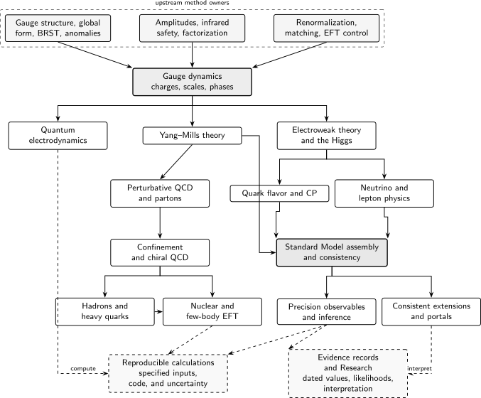
Across both branches, keep the question precise. Oscillations determine mass-squared differences, not the absolute neutrino mass. A confinement diagnostic in one theory does not prove a general Yang–Mills construction theorem. A fitted deviation requires an observable definition, correlations, and competing explanations before it supports a new interaction.

Where to go next

Use Perturbative QFT and Scattering for the amplitude and observable methods behind a particle calculation, or Renormalization and Effective Field Theory to develop matching and controlled expansions. For nonperturbative hadronic inputs, continue to Lattice and Hamiltonian QFT. Follow the relevant Research discussion when the question concerns a current measurement or unsettled interpretation; the theoretical criteria here apply independently of a particular data release.

References

• Pich, Antonio. “The Standard Model of Electroweak Interactions.” Proceedings of the 2010 European School of High-Energy Physics, CERN-2012-001 (2012), 1–50. arXiv:1201.0537v1. The cited locator uses the printed pagination of this preprint.