Conformal Field Theory and Bootstrap

Conformal field theory (CFT) studies quantum fields whose correlation functions respect conformal symmetry. It describes many critical points and supplies a nonperturbative language for quantum dynamics: specify local operators, their scaling dimensions, and their interaction coefficients, then ask whether they can belong to one consistent theory. The conformal bootstrap makes that question calculable by comparing different expansions of the same correlation function. This volume develops the underlying geometry and representations, exact low-dimensional examples, and analytic and numerical methods, with extensions to defects, thermal states, and protected sectors. Scale invariance alone is not assumed to imply conformal invariance.

Where to begin

• First study: start with Conformal Symmetry and Representations, then radial quantization and correlators. The first destination is a four-point crossing equation whose terms and positivity assumptions you can explain.
• A concrete laboratory: use Conformal Field Theory in One Dimension for a manageable crossing problem, or Two-Dimensional CFT: Algebraic and Rational Core for Virasoro symmetry and exact models.
• A research calculation: enter Numerical Bootstrap to formulate a bound, or Analytic and Lorentzian Bootstrap to extract data from causal limits. First fix the correlator, symmetry sectors, and spectrum assumptions using Chapter 3.

Helpful background. The Wilson OPE supplies local operator products; Reflection Positivity explains positive state norms; Linearized RG Flow connects fixed points to deformations; Multiplets and Selection Rules supplies representation language.

Chapters

1. Conformal Symmetry and Representations — Build the algebra, primary representations, descendants, and unitarity bounds.
2. Radial Quantization and State–Operator Correspondence — Turn operator insertions into states and compute their norms.
3. Correlators, OPE, and Conformal Blocks — Assemble correlation functions from conformal families and impose crossing.
4. Conformal Field Theory in One Dimension — Study ordering, exact blocks, and solvable crossing problems.
5. Two-Dimensional CFT: Algebraic and Rational Core — Connect Virasoro and affine symmetry to fusion, characters, and sewing.
6. Nonunitary, Logarithmic, Noncompact, and Nonrational Two-Dimensional CFT — Determine what changes when positivity, diagonalizability, or a discrete spectrum fails.
7. Higher-Dimensional CFT and Controlled Regimes — Use free theories and controlled expansions to organize interacting conformal data.
8. Boundaries, Defects, and Interfaces — Relate bulk and defect operators through their own consistency equations.
9. Weyl Anomalies, Deformations, and Flow Constraints — Study curvature response, perturbations, conformal manifolds, and RG constraints.
10. Numerical Bootstrap — Translate crossing into optimization problems with explicit approximation and verification checks.
11. Analytic and Lorentzian Bootstrap — Recover operator data using lightcone limits, inversion, and dispersion relations.
12. Energy Flow, Light-Ray Operators, and Conformal Colliders — Connect local CFT data to normalized energy detectors and causal constraints.
13. Modular and Thermal Bootstrap — Distinguish torus modular consistency from thermal correlation-function constraints.
14. Superconformal Bootstrap Interfaces — Combine supersymmetric protected data with superconformal crossing.
15. Large-N, Mellin, and Holographic CFT Interfaces — Organize factorization and Mellin amplitudes while keeping bulk interpretations conditional.

How the ideas connect

Consider four identical Hermitian scalar operators in a reflection-positive Euclidean CFT, at separated points. Radial quantization surrounds two insertions with a sphere. Expanding the state on that sphere into primary states and descendants gives the operator product expansion (OPE); its convergence follows from the Hilbert-space expansion when the sphere separates those insertions from the others. Each primary and all its descendants contribute one conformal block. This is why the algebra and state space come before a bootstrap calculation. See Pappadopulo et al. 2012, §2, pp. 7–8, Open PDF.

For an orthonormal, discrete primary spectrum, the unknown coefficients multiplying these blocks are squared real OPE coefficients and hence nonnegative. Exchanging the insertion pairs produces another channel for the same four-point function. Crossing requires the two sums to agree; positivity restricts which sums are possible. A continuous spectrum instead requires the appropriate spectral integral. The definitions and normalized equations are developed in Crossing Equations and Positivity.

This gives a practical exclusion test. Propose a spectrum, then seek a linear functional that is nonnegative on every allowed nonidentity crossing contribution and positive on the identity contribution. Applying it to the crossing equation would give a positive quantity equal to zero, so a verified functional excludes the proposal. Failure to find one does not construct a CFT. Finite computations must control block approximations, truncations, and numerical errors before their exclusions support the claimed bound. Simmons-Duffin 2017, §10.4, pp. 54–55, Open PDF explains this separation argument.

The remaining chapters change the available structure or the observable. Two-dimensional algebras organize additional descendants; nonunitary theories require a replacement for positive norms. Defects introduce new operator expansions. Lorentzian methods require a specified ordering, continuation sheet, and growth assumptions. Modular consistency constrains torus data, whereas thermal KMS relations constrain a chosen equilibrium state. Protected supersymmetric inputs and large-N limits can strengthen a problem, but an allowed numerical island does not prove existence or unique model identification, and large-N factorization alone does not establish a local gravitational dual.

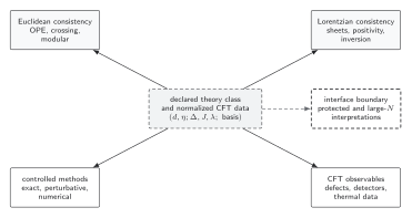
The optional data-and-consistency map (SVG) summarizes these branches: declared theory and normalized data supply Euclidean consistency, Lorentzian consistency, controlled methods, and CFT observables. Its dashed interface marks where protected or large-N interpretations require further assumptions. It is schematic, not a compulsory reading order.

Use the site’s conventions together with the local operator and block normalizations. Rescaling an operator changes its OPE coefficients; continuing a Euclidean expression changes its branch data. Compare invariant correlators or norms before combining formulas from different sources.

Detailed conventions and translation checks

The shared starting choices below accompany the relevant topic pages. Any override must state the conversion and reproduce an invariant quantity.

Axis	Shared convention	Required translation check
Lorentzian signature	$\eta_{\mu\nu}=\operatorname{diag}(+,-,\ldots,-)$	scalar product and $i\epsilon$ prescription agree
Euclidean continuation	positive $x_E^2$ with continuation path stated for Lorentzian use	same ordered boundary value is recovered
Conformal algebra	$[D,P_\mu]=P_\mu$, $[D,K_\mu]=-K_\mu$, $[K_\mu,P_\nu]=2\delta_{\mu\nu}D-2M_{\mu\nu}$	a Casimir eigenvalue or Jacobi identity agrees
Radial adjoint	$D^\dagger=D$, $P_\mu^\dagger=K_\mu$, $M_{\mu\nu}^\dagger=-M_{\mu\nu}$ in the no-$i$ generator convention	level-one and scalar level-two Gram norms agree
Scalar two-point function	unit coefficient, $(x^2)^{-\Delta}$	rescaling is inverted in every OPE coefficient
Degenerate operators	positive two-point matrix retained until a declared whitening	basis-invariant quadratic OPE weight agrees
OPE coefficient	coefficient multiplies a unit-normalized primary and its fixed descendants	a two- or three-point function round-trips
Cross ratios	$u=z\bar z$, $v=(1-z)(1-\bar z)$ with channel and ordering stated	all six permutation images agree
Scalar block	leading $12$-channel behavior $g_{\Delta,\ell}\sim u^{\Delta/2}$ with angular tensor declared locally	Casimir and OPE-limit checks agree
One-dimensional block	$g_\Delta(z)=z^\Delta{}_2F_1(\Delta,\Delta;2\Delta;z)$	series, integral, and Casimir forms agree
Two-dimensional stress tensor	$T(z)T(0)\sim(c/2)z^{-4}+2T(0)z^{-2}+\partial T(0)z^{-1}$	plane–cylinder shift and character vacuum energy agree
Four-dimensional stress tensor	$\langle TT\rangle=C_T\mathcal I/x^8$ and $C_T=40c/\pi^4$ in the displayed anomaly convention	a free-field anchor agrees
Weyl anomaly in 4D	$\langle T^\mu{}_{\mu}\rangle=(cW^2-aE_4+b\nabla^2R)/(4\pi)^2$	$S^4$ gives $dF/d\log R=-4a$
Fourier transform	$\widetilde{\mathcal O}(p)=\int d^dx\,e^{+ip\cdot x}\mathcal O(x)$, inverse phase $e^{-ip\cdot x}$ and measure $d^dp/(2\pi)^d$	position/momentum Ward identity round-trips
Discontinuity	$\operatorname{Disc}f(x)=f(x+i0)-f(x-i0)$; dDisc phases declared on the page	a frozen continuation path gives the same result
Modular variable	$q=e^{2\pi i\tau}$ with spin structure, vacuum shift, and sector sum explicit	$S$ and $T$ actions close in the chosen sector basis
Numerical output	crossing basis, derivative order, precision, approximation, feasibility sign, and solver version stated	independent residual and certificate agree
Mellin or detector data	contour/measure/normalization and Regge or smearing domain declared locally	pole residues or total-energy sum rule agrees

Where to go next

Use Renormalization and Effective Field Theory to follow deformations away from a fixed point; Supersymmetry and Duality to derive protected inputs; or Holography and Quantum Gravity to investigate the additional conditions behind a bulk description. The conformal-bootstrap research map supplies dated developments after the method and its assumptions are understood.

References

• Pappadopulo, Duccio, Slava Rychkov, Johnny Espin, and Riccardo Rattazzi. “OPE Convergence in Conformal Field Theory.” Physical Review D 86 (2012): 105043. DOI; Open PDF, arXiv:1208.6449v3.
• Simmons-Duffin, David. “TASI Lectures on the Conformal Bootstrap.” In New Frontiers in Fields and Strings, edited by Joseph Polchinski, Pedro Vieira, and Oliver DeWolfe, 1–74. World Scientific, 2017. DOI; Open PDF, arXiv:1602.07982v1. Page locators refer to the preprint.