Lattice and Hamiltonian QFT

Lattice and Hamiltonian methods make quantum field theories accessible beyond a weak-coupling expansion. A spacetime lattice turns a functional integral into a regulated statistical problem; a Hamiltonian formulation instead represents states and their evolution. Both approaches can reveal spectra, matrix elements, and dynamics that perturbation theory cannot reliably reach.

A useful organizing problem is to determine a particle mass from a Euclidean correlation function and reproduce it with a Hamiltonian calculation. Agreement becomes meaningful when the two calculations describe the same theory, use matched physical parameters, and control their different cutoffs. This volume teaches both the computational methods and the reasoning that connects their finite answers to continuum observables.

Where to begin

• First nonperturbative calculation: start with Lattice Regulators and Target Continuum Theories, then Euclidean Correlators and Spectral Information. The free scalar provides an exact reference before sampling an interacting theory.
• Hadronic spectra and scattering: enter through Links, Plaquettes, and Gauge Invariance if the regulator basics are familiar. Add fermions, statistical inference, and finite-volume amplitude methods as your observable requires.
• Real-time or variational physics: begin with Regulated Hamiltonian Field Theory. Choose a basis, tensor representation, or quantum encoding only after fixing the physical Hilbert space and target observable.

Helpful background. Regulated bosonic field integrals explains the Euclidean measure; Hamiltonian field theory supplies canonical initial data; probabilistic convergence and limit theorems supports sampling and uncertainty estimates.

Chapters

1. Lattice Regulators and Continuum Targets — Specify finite variables, boundaries, parameters, and the limits defining the desired continuum theory.
2. Lattice Observables and Continuum Inference — Extract spectra and matrix elements, renormalize operators, set scales, and extrapolate matched observables.
3. Lattice Gauge Theory — Build gauge-invariant link actions and distinguish loop, topology, flow, and gauge-fixed observables.
4. Lattice Fermions and Chirality — Understand doubling and the tradeoffs among chirality, locality, flavor, and numerical cost.
5. Sampling Algorithms for Lattice Fields — Construct and test algorithms that sample the intended measure.
6. Statistical Inference and Error Budgets — Account for correlations, equilibration, covariance, fit choices, and systematic uncertainty.
7. Finite-Volume Spectra and Amplitudes — Relate discrete energy levels to scattering under explicit channel, range, and symmetry assumptions.
8. Finite Density and Sign Problems — Diagnose complex-weight cancellations and the validity and limitations of proposed methods.
9. Hamiltonian Lattice Field Theory — Construct constrained Hilbert spaces and controlled spatial, local-state, and real-time limits.
10. Light-Front QFT — Develop bound-state calculations while controlling zero modes, currents, counterterms, and longitudinal cutoffs.
11. Hamiltonian Truncation and Variational Methods — Determine how omitted states affect energies and operators, then test cutoff convergence.
12. Tensor-Network QFT — Represent entangled states while separating bond, contraction, optimization, time, and continuum errors.
13. Quantum Simulation of QFT — Connect an encoded Hamiltonian, state preparation, evolution, and measurement to a verified field-theory observable.

How the ideas connect

A mass from a Euclidean correlator

Take a zero-momentum Hermitian operator $O$ in a finite spatial box. Assume a positive transfer operator and take the zero-temperature limit. After subtracting its vacuum expectation value, its correlator has the spectral form

$$C(t)=\sum_{n>0}|Z_n|^2e^{-\Delta E_n t}, \qquad Z_n=\langle0|O|n\rangle, \qquad \Delta E_n=E_n-E_0.$$

Here $t>0$ is Euclidean time and the states are unit normalized. Large time suppresses higher energies: if an isolated lowest contributing state has nonzero overlap, the correlator approaches a single exponential. The corresponding logarithmic ratio, divided by the time spacing, estimates its energy gap. Lepage 2005, § 2.2, pp. 5–6, Eqs. (23)–(26), PDF develops this mechanism in a quantum-mechanical example.

The inference is more demanding than fitting an exponential. Excited states matter at short times, statistical noise grows at long times, and finite temporal extent adds backward and thermal propagation. Different operator bases and fit windows test state isolation. A finite-volume level is not automatically a stable particle mass; scattering states and resonances need the finite-volume methods of Chapter 7.

From a finite answer to the target theory

The physical mass is not the bare mass inserted into the action. Along a continuum sequence, tune independent renormalized quantities and measure a dimensionless comparison such as a mass ratio. If the spatial spacing is $a$ and the box has $N$ sites per direction, its size is $L=Na$. Sending $a$ to zero at fixed $N$ shrinks the box; a continuum limit at fixed physical $L$ instead increases $N$. Volume dependence must then be controlled separately.

A Hamiltonian calculation can target the same spectrum, but its basis cutoff or local Hilbert-space truncation creates an additional error. Tensor methods add bond and contraction errors; real-time calculations add time-step and observation-window effects; quantum devices add preparation, encoding, and measurement errors. Refining one does not remove the others. Independent formulations are strongest checks when their dominant approximations differ.

These observations organize every route as a sequence: define the finite problem, map its operators to the physical observable, vary independent errors, compare an exact or independent reference, and take explicitly ordered limits. The optional formulation map (SVG) displays these steps for Euclidean, Hamiltonian, light-front, truncation, tensor, and quantum-simulation routes. A valid endpoint is a renormalized observable, expressed as a dimensionless ratio when comparison requires a reference scale.

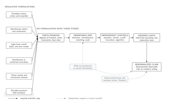
The detailed target and regulator comparison supplies the reusable specification with a free-scalar example: fields, measure, geometry, action, symmetries, tuning, operator normalization, scale hierarchy, held-fixed quantities, and independent checks. Use it before interpreting an apparently converged computation as a result for the intended theory.

Where to go next

Continue to Gauge Theories and the Standard Model for the hadronic quantities these methods compute, or Many-Body QFT and Quantum Matter for lattice models, phases, and response. Renormalization and Effective Field Theory explains cutoff dependence and matching. For proof-level existence and reconstruction questions, consult Mathematical QFT; a successful numerical extrapolation and a construction theorem establish different kinds of result.

References

• Lepage, G. Peter. “Lattice QCD for Novices.” Lectures at HUGS 1998, published in J. L. Goity (ed.), Strong Interactions at Low and Intermediate Energies, World Scientific (2000), 49–90. arXiv:hep-lat/0506036v1, posted 2005. The cited locator uses the printed pagination of this preprint.