Thermal and Nonequilibrium QFT

Thermal and nonequilibrium QFT studies quantum fields in states with temperature, density, preparation history, driving, or environmental exchange. The central question is how microscopic quantum dynamics produces collective behavior: screening, diffusion, viscosity, phase conversion, or relaxation toward equilibrium. Different questions require different descriptions. An equilibrium partition function, a real-time correlation function, a kinetic equation, and a fluid theory retain different information. This volume teaches how to choose among them and how to derive their connections without losing the assumptions that make each useful.

Where to begin

• First study of thermal fields: start with Equilibrium States, Ensembles, and Thermodynamic Limits, then KMS states, thermal perturbation theory, and resummation. Aim to compute a static observable while recognizing an uncontrolled infrared approximation.
• A time-dependent quantum state: enter Real-Time Contours, Keldysh Bases, and Response, then two-time evolution in Chapter 8. Choose kinetic, stochastic, or open-system reductions only after identifying the relevant separation of timescales.
• Transport or plasma applications: begin with Hydrodynamic Variables, Frames, and Ideal Modes and Response, Transport, and Inference. Chapters 12 and 17–18 connect constitutive theories to hot gauge matter and collision observables.

Helpful background. Partition Functions and Thermodynamic Response supplies equilibrium derivatives; Closed-Time-Path Grammar supplies in–in evolution; Beta Functions and Running Parameters and Power Counting explain scale dependence and controlled truncation.

Chapters

1. Equilibrium States, Ensembles, and Thermodynamic Limits — Define ensembles, static response, fluctuations, and thermodynamic phases.
2. KMS States, Imaginary Time, and Thermal Spectra — Connect equilibrium to imaginary-time boundary conditions and spectral representations.
3. Finite Density and Conserved Charges — Introduce chemical potentials, charged states, and density-dependent access limitations.
4. Thermal Perturbation Theory and Renormalization — Compute thermal corrections and diagnose the infrared failure of naive perturbation theory.
5. Thermal EFT, Screening, and Resummation — Separate thermal scales and match effective descriptions without double counting.
6. Thermal Phases, Metastability, and Nucleation — Distinguish equilibrium phase criteria from the dynamics and rates of phase conversion.
7. Real-Time Contours, Keldysh Bases, and Response — Generate causal responses while keeping initial states and contour normalization explicit.
8. Nonequilibrium Green Functions and Kadanoff–Baym Evolution — Evolve two-time correlators with controlled self-energy and memory approximations.
9. Critical and Stochastic Dynamics — Relate noise, dissipation, slow modes, and dynamic critical behavior.
10. Kinetic Theory and Transport Equations — Derive distribution-function dynamics when quasiparticle and gradient approximations apply.
11. Hydrodynamic Variables, Frames, and Ideal Modes — Build collective dynamics from conservation laws and the correct slow variables.
12. Relativistic Dissipation, Transients, Stability, and Causality — Test constitutive formulations for stable and causal evolution.
13. Fluctuating, Generalized, and Schwinger–Keldysh Hydrodynamics — Include fluctuations, extra conserved quantities, and additional slow modes.
14. Response, Transport, and Inference — Define transport coefficients and distinguish response relations from inverse reconstruction.
15. Thermalization, Integrability Breaking, and Quantum Chaos — Separate equilibration, prethermal behavior, operator growth, and evidence for chaos.
16. Open QFT and Driven Dynamics — Derive reduced evolution and identify the limits of Markovian or master-equation descriptions.
17. Hot Gauge Theory and Plasma EFTs — Resolve hard, electric, magnetic, and transport scales in gauge plasmas.
18. QCD Matter and Multistage Collision Inference — Connect successive collision stages and probes to conditional statements about QCD matter.

How the ideas connect

A small disturbance of a conserved charge density provides a useful thread. Begin with a homogeneous equilibrium state and ask two questions: how much charge accumulates when its chemical potential changes, and how fast does an inhomogeneity relax? The first is a static susceptibility, determined from equilibrium response. The second requires dynamics.

In an isotropic normal phase, suppose the charge mode has a finite diffusion coefficient and decouples from every other slow mode at linear order. Its leading long-wavelength equation is

$$\partial_t\delta n=D\nabla^2\delta n, \qquad \omega=-iDk^2.$$

Here $\delta n$ is the charge-density disturbance, $D$ the diffusion coefficient, and $k$ the spatial wave number. A Fourier mode decays as $e^{-Dk^2t}$ for $D>0$; conservation makes the relaxation rate vanish as $k\to0$. The same mode appears as a pole of the retarded density correlator. This links a macroscopic equation to a microscopic response observable, as derived in Kovtun 2012, §2.1, pp. 16–18, Open PDF. The diffusion chapter page develops the conductivity–susceptibility relation and its coupled generalization.

The surrounding chapters answer different parts of that calculation. The equilibrium ensemble and Kubo–Martin–Schwinger (KMS) condition specify the state and relate its correlation functions. Imaginary-time methods provide equilibrium observables, but extracting a narrow transport feature from finite noisy Euclidean data is an inverse problem. Real-time contours retain the response and preparation information directly. Nonequilibrium Green functions can keep memory and coherence; kinetic equations discard some of that information under additional quasiparticle and gradient assumptions.

Hydrodynamics can apply even when a quasiparticle picture does not. It needs separation between slow collective modes and faster relaxation, with every relevant slow variable included. Near a critical point, an additional slowly relaxing field can invalidate the simplest fluid description. Stochastic theories restore fluctuations consistent with the coarse graining. For a subsystem exchanging information with an environment, an influence functional or master equation instead describes reduced dynamics; complete positivity alone does not establish that a Markov approximation is accurate.

The diffusion equation is a long-wavelength approximation, not a relativistic propagation law at arbitrary wave number. Its formal instantaneous spreading does not license extending it beyond that regime. Stability, causality, and the initial-value problem must be checked for the chosen relativistic formulation. Likewise, hydrodynamic behavior can emerge before isotropy or full thermalization; each statement concerns different observables.

Applications add their own scale and inference requirements. In weakly coupled hot non-Abelian gauge theory, temperature, electric screening, and magnetic scales require distinct treatment. A collision prediction also joins initial conditions, pre-equilibrium evolution, hydrodynamics, conversion to particles, and subsequent interactions. Agreement with data constrains that combined model and its uncertainties; it does not make an inferred transport parameter independent of those choices.

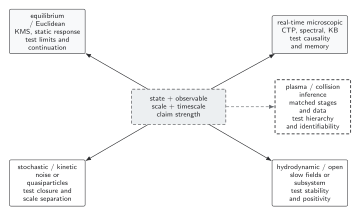
The optional description-and-regime map (SVG) summarizes the choices. State, observable, length scale, and timescale select equilibrium/Euclidean, microscopic real-time, stochastic/kinetic, hydrodynamic/open-system, or plasma/collision descriptions. Their respective checks concern limits and continuation; causality and memory; closure and scale separation; stability and positivity; or matching and parameter identifiability. These are alternative descriptions with overlapping domains, not a mandatory sequence. The map is schematic.

Where to go next

Use Many-Body QFT and Quantum Matter for transport and phases in material systems; Lattice and Hamiltonian QFT for controlled equilibrium and real-time computations; or Holography and Quantum Gravity for examples of strongly coupled thermal dynamics. The thermal and nonequilibrium research field collects dated developments and open questions.

References

• Kovtun, Pavel. “Lectures on Hydrodynamic Fluctuations in Relativistic Theories.” Journal of Physics A: Mathematical and Theoretical 45 (2012): 473001. DOI; Open PDF, arXiv:1205.5040v1. Page locators refer to the preprint.