Renormalization and Effective Field Theory

Renormalization relates the parameters and operators in a quantum field theory to finite, measurable predictions. Effective field theory (EFT) makes those predictions systematic within a specified range of energies, retaining the relevant degrees of freedom and organizing unresolved physics into interactions with an expansion in small parameters. Together they explain how a useful description can change with resolution while its physical predictions remain consistent.

The applications span precision particle calculations, critical phenomena, and low-energy effective descriptions. The questions are what to retain, how to determine parameters, how to compare scales, and how to estimate omitted terms.

Where to begin

• First study of renormalization: begin with local counterterms, then follow Chapters 2–3 through operator mixing and running. Aim for a finite prediction whose residual scale dependence begins beyond the retained order. The renormalization and RG primer gives a shorter introduction.
• Critical phenomena and continuum limits: begin with running in Chapter 3, then Chapters 4–5. Follow changes of resolution into theory space and identify the fixed points, perturbations, and evidence behind universality.
• An EFT calculation: begin with EFT construction, then Chapters 7–8 for matching and operator bases. Review Chapters 1 and 3 for renormalization and running; use Chapter 9 when several low scales require separate modes. The researcher pathway offers a focused route.

Helpful background. Review regulators and continuum limits to distinguish a computational regulator from a physical cutoff, and UV/IR poles in amplitudes to identify which singularities require ultraviolet subtraction. For operator mixing or symmetry constraints, use local insertions and quantum currents, respectively.

Chapters

1. Ultraviolet Renormalization and Locality — Why can ultraviolet divergences be absorbed into local counterterms, and how are finite parameters fixed by physical inputs?
2. Composite Operators and Mixing — How do local insertions renormalize together, including coincident-point terms and the compensating evolution of their coefficients?
3. Renormalization-Group Equations and Running — How does scale independence produce beta functions, anomalous dimensions, and the resummation of large logarithms?
4. Wilsonian and Functional Renormalization — How does integrating fluctuations change an action, and how are exact functional flows converted into controlled approximations?
5. Fixed Points, Universality, and Continuum Limits — How do flow directions determine scaling and crossover, and what establishes a continuum limit beyond a zero of a truncated beta function?
6. Effective Field Theory: Construction and Power Counting — Which fields and interactions are needed for a specified accuracy, and where does the expansion fail?
7. Matching, Decoupling, and Threshold Evolution — How are short-distance coefficients determined by comparing theories, and under which assumptions do heavy particles decouple?
8. Operator Bases and Field Redefinitions — Which interaction terms are redundant for the chosen observables, and how can bases be translated consistently?
9. Modes, Factorization, and Multiscale RG — How can several momentum scales be separated without double counting, with compatible virtuality and rapidity evolution?
10. Effective-Theory Architecture Atlas — Which EFT structure suits a chiral, heavy-particle, nonrelativistic, gravitational, or open-system problem?
11. Naturalness, Scale Sensitivity, and Emergence — What do calculable scale sensitivity and symmetry protection establish, and which further conclusions depend on assumptions or interpretive choices?

How the ideas connect

Consider light particles interacting through a heavy mediator of mass $M$, at external momenta and light masses of order $Q\ll M$. The mediator’s exchange can be expanded into local light-field interactions and derivative corrections. Power counting decides which terms and loops are needed for the desired accuracy. Light fields still propagate and fluctuate: replacing the mediator does not make the effective theory classical.

Renormalization supplies the local counterterms needed for those loops and defines finite inputs. Matching then compares full- and effective-theory amplitudes in their common low-energy domain. Both sides contain the same infrared physics; subtracting it consistently isolates the short-distance coefficients. Running transports those coefficients from a matching scale near $M$ toward $Q$, resumming logarithms of the hierarchy. These are distinct steps, illustrated explicitly in Manohar 2018, §§ 5.5–5.9, pp. 38–45, PDF. When no microscopic theory is known, EFT coefficients can instead be inferred from measurements or nonperturbative calculations.

Keep three scales distinct. Removing an auxiliary ultraviolet regulator holds the renormalized inputs fixed. Changing the subtraction scale $\mu$ redistributes contributions between parameters, operators, and loop corrections; their complete physical combination stays unchanged. At finite order, residual dependence should begin beyond the retained accuracy. Lowering a Wilsonian scale $k$ integrates out fluctuations and changes the action for the remaining modes while preserving their low-momentum predictions. The effective average action, which generates scale-dependent one-particle-irreducible vertices, is a related but distinct object. Exact flow equations still require approximations in practical calculations; regulator dependence and enlarged truncations help test those approximations. See Dupuis et al. 2021, §§ 2.1.2–2.2, pp. 8–9, PDF.

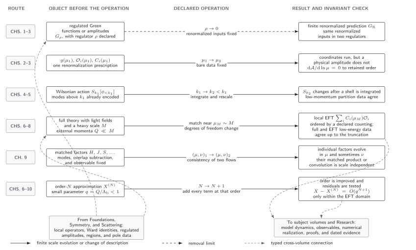
Two further operations extend this picture. Factorization separates momentum modes that coexist in an observable: overlapping regions must be subtracted, and dependence on $\mu$ and any auxiliary rapidity scale $\nu$ must cancel between the factors to the claimed order. Improving the approximation adds every contribution required by the next retained order. Residual scale variation tests missing perturbative terms; it does not by itself measure omitted powers of $Q/M$. Finite changes of scheme or operator basis likewise require translating coefficients before comparing predictions.

The optional scale-operation map (full-size SVG) summarizes these six operations and their checks. Read its rows as changes of description, not as positions on one energy axis; it is schematic. Its incoming connections supply operators, symmetry identities, and regulated amplitudes, while its outgoing connections lead to the applications below.

Where to go next

• For a process and a measured rate, continue to Perturbative QFT and Scattering; for QED, QCD, or Standard Model coefficients and applications, use Gauge Theories and the Standard Model.
• For fixed-point correlation functions and scaling data, continue to Conformal Field Theory and Bootstrap; for phases and collective excitations, use Many-Body QFT and Quantum Matter.
• For numerical continuum extrapolation and nonperturbative operator evolution, continue to Lattice and Hamiltonian QFT; for theorem-level control of a continuum construction, use Mathematical QFT.

References

• Dupuis, Nicolas, Léonie Canet, Astrid Eichhorn, Walter Metzner, Jan M. Pawlowski, Michel Tissier, and Nicolás Wschebor. 2021. “The Nonperturbative Functional Renormalization Group and Its Applications.” Physics Reports 910: 1–114. DOI. Open PDF, arXiv:2006.04853v3; page locators above refer to this version.
• Manohar, Aneesh V. 2018. “Introduction to Effective Field Theories.” Lectures at the Les Houches summer school Effective Field Theory in Particle Physics and Cosmology, 2017. arXiv:1804.05863v1. Open PDF; page locators above refer to this version.