Many-Body QFT and Quantum Matter

Many-body quantum field theory explains how interacting particles become quantum fluids, magnets, metals, insulators, and other collective forms of matter. Its central objects are low-energy fields, correlation functions, and response: they connect a microscopic Hamiltonian to excitations and to quantities a probe can measure.

This volume follows that connection across gases, electronic and spin systems, topology, disorder, and nonequilibrium dynamics. A dilute Bose gas offers a first example: matching two-body scattering fixes an effective interaction, fluctuations about a condensate produce sound, and density response makes the collective mode observable. More strongly correlated systems require different variables and different forms of control.

Where to begin

First graduate study: begin with Galilean Fields, Scales, and Low-Energy Degrees of Freedom, then Many-Body Correlators, Response, and Quasiparticles. Use Bose and Fermi fluids to learn how fields become physical predictions.
Strong correlations and phases: enter through Correlated Lattice Fermions and Mott Physics if the operator and response language is familiar. Continue toward magnetism, criticality, or topological matter according to the degrees of freedom and diagnostic.
An experimental or numerical result: start with From Measured Intensity to Many-Body Claim, then consult the relevant system chapter. Identify which correlator is measured and which alternative explanations must be tested.

Helpful background. Canonical quantization and Fock space supply the operator language; symmetry realization supplies order parameters. Power counting controls low-energy expansions, while thermodynamic response and retarded correlators connect states to observables.

Chapters

Nonrelativistic Fields and Low-Energy Reduction — Translate particles, orbitals, and constraints into fields with a stated low-energy range.
Many-Body Correlators, Response, and Quasiparticles — Relate Green functions, self-energies, vertices, and spectral features to measurable response.
Resonant Interactions and Universal Quantum Gases — Use scattering data and few-body scales to define controlled many-body inputs.
Bose Quantum Fluids and Lattice Bosons — Develop condensation, collective modes, superfluid response, and interaction-driven phases.
Fermi Surfaces and Fermi Liquids — Build the low-energy description of fermions near a Fermi surface and test its breakdown.
Correlated Lattice Fermions and Mott Physics — Distinguish correlation-driven insulating behavior from band, magnetic, and disorder effects.
Pairing, Superfluidity, and Superconductivity — Connect pairing channels and collective order to stiffness, electrodynamics, and observables.
Quantum Impurities, Polarons, and Kondo Matter — Follow local degrees of freedom into screening, dressing, and collective behavior.
One-Dimensional Quantum Matter — Use bosonization and exact mappings when ordinary quasiparticle pictures fail.
Quantum Magnetism and Frustration — Derive spin models and diagnose order, collective fluctuations, and frustrated phases.
Quantum Phase Transitions and Critical Metals — Organize competing scales and test critical descriptions of bosonic and metallic systems.
Band Geometry and Symmetry-Protected Matter — Relate Berry geometry and symmetries to bulk invariants, boundaries, and response.
Fractional Quantum Hall Matter and Anyons — Connect projected interactions to intrinsic topological order, fractional charge, and statistics.
Fractionalization and Emergent Gauge Fields — Test constrained parton descriptions, gauge dynamics, and fractionalized excitations.
Disorder, Localization, and Glasses — Analyze randomness, diffusion, rare regions, and the limits of phase diagnostics.
Cold Atoms and Synthetic Matter — Match engineered platforms to Hamiltonians, interaction scales, and calibrated probes.
Integrable Quantum Matter and Generalized Hydrodynamics — Turn conserved charges and quasiparticle distributions into state and transport predictions.
Nonequilibrium, Driven, and Open Quantum Matter — Separate transient, prethermal, steady, and asymptotic behavior after driving or coupling to an environment.
Quantum-Matter Probes, Inference, and Evidence — Compare theory, computation, and experiment while tracking resolution, uncertainties, and competing explanations.

How the ideas connect

From atoms to sound

Consider a uniform three-dimensional Bose gas at zero temperature, with repulsive short-range interactions and gas parameter $na_s^3\ll1$ . Here $n$ is particle density and $a_s>0$ the scattering length. At leading order the matched coupling is $g=4\pi a_s/m$ for particle mass $m$ in natural units. Quadratic fluctuations about condensate density $n_0$ have dispersion

E_k=\sqrt{\epsilon_k(\epsilon_k+2gn_0)}, \qquad \epsilon_k=\frac{k^2}{2m}.

The same mode is sound at small momentum, $E_k\simeq ck$ with $c=\sqrt{gn_0/m}$ , and approaches particle-like behavior when kinetic energy dominates. Both statements apply below the interaction-range cutoff. These limits follow directly from the square root; the gap closes as required for the phase mode. Dalfovo et al. 1998, § IV.A, pp. 18–19, Eqs. (65)–(71), PDF derives the spectrum and its sound limit.

This example connects microscopic matching, the condensate approximation, collective excitations, and response. The Bogoliubov calculation checks the mode’s normalization and density response; depletion tests the approximation’s self-consistency. Strong interactions, low dimension, or proximity to a transition require a different treatment. Condensation and superfluid response are distinct properties, so identifying one does not by itself measure the other.

From a model to evidence

The organizing sequence remains useful outside dilute gases: specify microscopic degrees of freedom and constraints; derive the retained low-energy variables; fix the state, dimension, and regime; calculate excitations and a normalized response; then compare with numerical or experimental evidence. The optional volume map (SVG) depicts this sequence and its links to general methods, reproducible calculations, and dated Research; its structured description (JSON) preserves the same relationships.

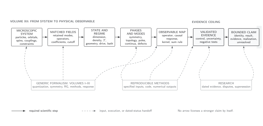
Each step can change the appropriate question. A band invariant does not by itself imply intrinsic topological order. A parton mean-field state needs projection and gauge-dynamics checks before it describes a physical spin liquid. A numerical crossing needs size and cutoff studies before it locates a thermodynamic phase boundary. A spectral peak needs a probe model, linewidth, and alternatives before it identifies a quasiparticle. The evidence comparison below keeps these different conclusions separate.

Evidence classes and the limits of a conclusion

Evidence fixes the ceiling of the conclusion

The following table gives the volume-wide evidence classes and their claim ceilings. It is not a strict total order: theorem, numerical, experimental, and platform evidence can form partly independent branches. Moving from a model-side statement toward a platform, material, or mechanism claim adds the obligations on the relevant branches; no row follows automatically from the one above it.

Evidence level	What may be concluded	Required support	What it does not establish
Exact identity or theorem	The stated relation holds under its definitions and hypotheses	derivation or theorem with domains, state, limits, and conventions	applicability to a material, uncontrolled approximation, or different limit
Controlled calculation	An observable has a stated expansion or error in a declared regime	power counting, remainder or convergence evidence, and independent checks	behavior beyond the control window
Effective-description result	A low-energy model reproduces specified observables over a calibrated range	matching data, retained symmetries, breakdown scale, and negative tests	unique microscopic origin or universal phase identity
Numerical phase evidence	Finite representations support or disfavor candidate phases	symmetry sectors, cutoff and size sequences, solver errors, drift, and competing diagnostics	a thermodynamic phase boundary from one crossing or cluster
Experimental response evidence	A normalized response feature is present within stated uncertainty	probe matrix element, resolution, background, covariance, reproducibility, and alternatives	unique quasiparticle, order, topology, or mechanism from one feature
Platform realization evidence	A device or atomic system implements and probes an effective Hamiltonian in a calibrated window	preparation, scale hierarchy, loss/heating/control errors, and observable validation	exact realization outside the window or equivalence to a target material
Model-phase identification	A specified Hamiltonian or field theory has the stated phase under declared limits	a theorem or converged complementary diagnostics, phase-boundary control, and exclusion of viable model phases	realization of that phase in a platform or material
Platform, material, or mechanism attribution	Multiple independent observations favor a specific realization or mechanism over viable alternatives	calibrated model-to-system matching, joint comparison, shared-systematic accounting, predictive and null tests, and a supersession record	certainty stronger than the weakest analytic, numerical, or experimental input

Download the structured evidence-class table (JSON), which preserves the scoped columns, row order, qualifications, and limits of interpretation.

Where to go next

Use Thermal and Nonequilibrium QFT for general response, kinetics, and open-system methods, and Lattice and Hamiltonian QFT for numerical representations and convergence. Quantum Information in QFT develops information-based diagnostics. For changing material, platform, or mechanism claims, consult Research: Quantum Matter and Emergence alongside the durable theory.

References

Dalfovo, Franco, Stefano Giorgini, Lev P. Pitaevskii, and Sandro Stringari. “Theory of Bose–Einstein Condensation in Trapped Gases.” Reviews of Modern Physics 71 (1999), 463–512. DOI. Open PDF: arXiv:cond-mat/9806038v2 (1998). The cited locator uses this preprint’s printed pagination.