

Large-N Limits, Normalizations, and Orders of Limits
A nontrivial large- limit is defined by an index family, a normalization of the action and fields, the couplings and operator normalizations held fixed, a state, and an order of limits. There is no universal instruction to “send to infinity.” Vector, matrix, gauge, and tensor theories keep different interactions finite, select different graph families, and can fail for different infrared or critical reasons.
Required background. What does nonperturbative mean? supplies the observable, regulator, and control data that must accompany a limiting claim. Running couplings and dimensional transmutation supplies the distinction between a bare -scaling and a renormalized coupling held fixed at a declared scale.
Helpful background. The O(N) model as a strong-coupling laboratory supplies a physical vector-model application.
The data that define a large-N limit
Section titled “The data that define a large-N limit”Throughout this chapter, an index written is a vector index, a pair is an adjoint or matrix index, and is a rank-three tensor with each of . Unless a page says otherwise:
- the regulator, spacetime manifold, boundary conditions, state, and renormalization scale are fixed before the limit;
- the renormalized parameters named below are held fixed at ; they need not be dimensionless;
- invariant operators are normalized so their one-point functions remain ;
- connected correlation functions are taken in one selected phase or clustering state;
- volume, continuum, critical, and infrared limits are written in their intended order.
These choices are part of the mathematical statement. Changing any one of them can change the power of or the leading saddle.
Four representative Euclidean actions make the distinction concrete, with weight . The index counts are formal Wick expansions about a regulated, invertible Gaussian, after gauge fixing where needed. An actual functional integral additionally requires a specified stable potential or integration cycle. In engineering mass dimensions, for the quartic vector, tetrahedral tensor and gauge couplings below, while for the matrix couplings. Holding these parameters fixed is an -scaling prescription at fixed , not a claim of scale invariance.
For an vector field,
with held fixed. Components have propagators, a quartic vertex contributes , and every closed vector-index loop contributes .
For a Hermitian matrix field,
with every fixed. The Gaussian contraction is
Thus a ribbon propagator contributes , a single-trace vertex contributes , and every closed index face contributes .
For Yang–Mills, choose and absorb the coupling into the connection, so and :
The ’t Hooft coupling is held fixed. Adjoint propagators and vertices have the same overall and weights as above, but the exact color projector is
The first term gives the oriented matrix strands; the traceless subtraction must be retained for exact finite- color factors. The usual ribbon organization describes the leading color flow and its resolved corrections, not an equality between the full covariance and the Hermitian-matrix covariance. With fundamental flavors, the standard ’t Hooft limit also holds fixed; a fundamental loop makes a boundary and is suppressed by relative to a closed adjoint surface. The Veneziano limit instead keeps fixed and is a different expansion.
For the tensor example used here, take a real field with a Gaussian propagator of order one and the tetrahedral interaction
with fixed. A vertex contributes and each single-color closed strand contributes . Here the bosonic model is a formal Gaussian expansion: the tetrahedral potential is generally not positive definite, so this expression alone does not define a stable real Euclidean measure. It is the commuting version of Klebanov and Tarnopolsky 2017, arXiv v5, § 1, Eqs. (1.3)–(1.4), HTML, with their coupling equal to . This is one model-specific tensor scaling, not a universal rule for all tensor invariants.
Large-N counting and topology map
Section titled “Large-N counting and topology map”The figure compares the four counts. In its matrix panel, dashed circles mark the cyclic order of one vertex’s slots and solid chords mark Wick pairings. Both representatives have and ; their different index-boundary counts give different genera after capping. The tensor panel shows an exponent-preserving insertion; the separate dominance argument is stated below. The bottom panel removes the matrix action’s overall and changes the graph powers.
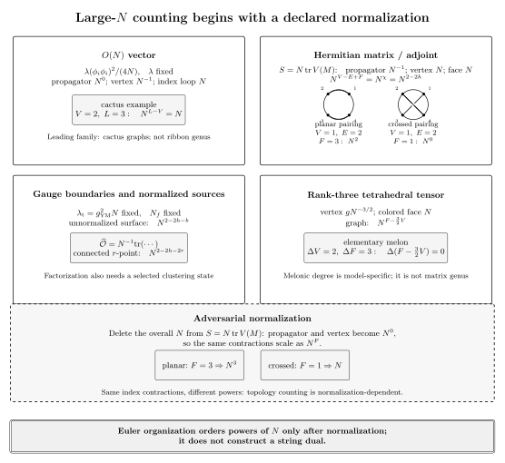
Powers of follow from the stated propagator, vertex and index-loop factors. Dashed circles mark cyclic slot order; solid chords are Wick pairings, and their crossing adds no vertex. After thickening and capping the index boundaries, both planar quartic pairings have , , ; the crossed pairing has . One planar representative is drawn. Gauge counting uses leading color flow; the formal tensor example preserves an exponent without proving dominance. The matrix counts are exact and the diagrams are schematic; counting alone does not construct a string dual.
For a connected vacuum ribbon graph with single-trace vertices, propagators, and closed index faces,
Thickening a Hermitian-matrix ribbon graph produces an orientable surface with boundary, which retracts onto the graph and has Euler characteristic . Capping each of its closed index boundaries with a disk produces a closed surface, so
where is the genus. If unnormalized fundamental or source boundaries are present, leave those specified boundaries uncapped:
An explicit factor in each normalized trace operator supplies a further . Consequently, for
the planar connected -point function scales as
Label the four cyclic slots . The pairings and are planar; is crossed. The two topological types have the counts
in the canonical matrix normalization. If the same written matrix field is instead assigned
with no overall , propagators and vertices are both . The powers become : for the planar pairing and for the crossed pairing. This is a counterexample to normalization-blind topology counting.
The formal Hermitian Wick expansion and its genus organization are developed in Di Francesco, Ginsparg and Zinn-Justin 1994, § 1.2, printed preprint pp. 7–10, PDF. They organize powers of ; by themselves they do not construct a worldsheet measure, establish target-space locality, identify the complete spectrum, or prove a string dual.
Large-N scaling comparison
Section titled “Large-N scaling comparison”The table is a semantic counterpart to the figure and fixes the conventions reused throughout the chapter.
| Family or claim | Indices, action, and held data | Elementary count | Normalized observable and leading scaling | Required limit or failure test |
|---|---|---|---|---|
| O(N) vector | φᵢ; interaction λ(φᵢφᵢ)²/(4N); hold λ fixed | Propagator N⁰; vertex N⁻¹; closed index loop N; graph N^(L−V) | Q̂ = N⁻¹φᵢφᵢ = O(1); leading vacuum and cactus graphs are O(N) | Check L = V + 1 for the proposed leading family and verify that infrared or critical enhancements do not offset 1/N |
| Hermitian matrix | Mⁱⱼ; S = N tr V(M); hold all single-trace couplings gₖ fixed | Propagator N⁻¹; vertex N; face N; graph N^(V−E+F) | Ôₖ = N⁻¹ tr Mᵏ = O(1); a connected r-point function is O(N^(2−2r)) at genus zero | For the zero-dimensional Hermitian integral, verify W(z) ∼ 1/z, density normalization and positivity, support choice, and distance from a critical edge |
| Adjoint gauge | Aij; S = N/(2λt) ∫ tr F²; hold the renormalized λt = gYM2N fixed | Double-line propagator N⁻¹; interaction vertex N in the stated convention; adjoint face N | N⁻¹ tr F² and normalized Wilson loops are O(1); connected invariant correlators are suppressed | Fix gauge group, generator trace, matter representation, Nf scaling, state, regulator, and μ before counting |
| Fundamental-matter boundary | Fundamental color line with Nf fixed | Each quark loop removes an adjoint face and contributes Nf; relative weight Nf/N | A disk-like unnormalized boundary is N¹ rather than the adjoint sphere's N² | If Nf/N is fixed instead, use the Veneziano expansion; do not quote fixed-Nf suppression |
| Rank-three tetrahedral tensor | Formal Gaussian expansion of Tabc with O(N)3; vertex gN−3/2; hold g fixed | Propagator N⁰; vertex N⁻³ᐟ²; colored face N; graph N^(F−3V/2) | N−3TabcTabc = O(1); leading connected vacuum graphs scale as N3 | Verify the invariant and covariance; melonic dominance is model-specific and is not a matrix-genus statement |
| Volume or orbifold equivalence | Compare only the common neutral sector at fixed ’t Hooft data | Factorization closes neutral loop equations only at leading N | Center-neutral, projection-invariant observables can agree at N = ∞ | Center and projection symmetries must be unbroken; declare translation realization and the N, volume, lattice-spacing, and continuum order |
For the vector row, set at the fixed regulator. Wick’s three pairings give
The vertex factor therefore leaves a leading and a subleading constant. More generally, a leading cactus routing has . In the figure’s example, a self-contracted pair at each vertex and two lines joining the remaining pairs leave three independent index sums, giving .
For the tensor row, inserting an elementary two-vertex melon adds three colored faces and two vertices:
This preserves an exponent; it does not prove dominance. For connected tadpole-free vacuum graphs of this invariant, the separate bound is , with saturation precisely for melonic graphs. The proof uses the Euler characteristics of the three two-color ribbon graphs, then recursively reduces a saturating graph through two-vertex subgraphs Klebanov and Tarnopolsky 2017, arXiv v5, § 2, Eqs. (2.1)–(2.7) and following argument, HTML.
Tadpoles in the bosonic expansion are subleading without changing the interaction. Use . At a common point , relabel its four factors as . Contracting the first pair gives
Each possible pair shares exactly one index, giving the same extra . Together with this is an quadratic insertion. Collapsing it removes one face and one vertex, lowering the original graph’s exponent by relative to the reduced graph. The terminal one-vertex vacuum has and scales as . Repeated removal and the tadpole-free bound thus exclude tadpoles from the leading vacuum power. This argument is at fixed perturbative order and fixed regulator with -independent Gaussian parameters; it supplies no uniform cutoff limit or convergence theorem. More developed tensor models belong to tensor large N, whose colored model has different field content.
Orders of limits are part of the result
Section titled “Orders of limits are part of the result”A complete statement should display an order such as
or explain why another sequence is required. The notation does not assert that the limits commute.
Important obstructions include:
- Continuum and . Bare couplings depend on the regulator and on . Compare theories at fixed renormalized and a fixed physical scale, not at the same unrenormalized symbol.
- Volume and symmetry breaking. A finite-volume symmetric state can be a mixture of phases. Factorization and saddle selection can change if , , and a symmetry-breaking source is removed in another order.
- Infrared and . A nominal correction multiplied by an infrared-divergent integral need not remain small as or a correlation length diverges.
- Matrix criticality. At fixed distance from a support transition, the genus expansion is ordered. Approaching the transition with can make all genera comparable and require a double-scaled variable.
- Volume reduction. Taking at fixed reduced volume is useful only while the center and projection symmetries remain unbroken and only for neutral observables Kovtun, Ünsal, and Yaffe 2007, §§2–4.
- Exponentially small sectors. Effects of order vanish at every fixed order in but can govern level splitting, saddle competition, or large-order behavior.
A simple mathematical witness is
Then
Pointwise large- control away from is not uniform near the boundary.
First application: vector versus ’t Hooft limits
Section titled “First application: vector versus ’t Hooft limits”The vector and gauge theories can both be called “large ,” but their surviving diagrams differ.
In the vector model, keep fixed in . A connected leading vacuum graph with quartic vertices and index loops scales as . The natural singlet is .
In gauge theory, keep fixed. Adjoint propagators carry two oriented strands, and a connected planar vacuum graph scales as regardless of its number of vertices. The natural local invariant is . Holding rather than fixed makes grow with and does not define the same perturbative reorganization.
The different powers reflect different numbers of degrees of freedom— versus —and different index combinatorics. Neither limit is more fundamental, and neither supplies the tensor scaling by analogy.
Common pitfalls
Section titled “Common pitfalls”Writing only the coupling that is held fixed. The same symbol can accompany different field and action normalizations. State the quadratic term, propagator, vertex, index-loop factor, and normalized observable.
Calling every trace a boundary without tracking its prefactor. A topological boundary changes the Euler characteristic, while an explicit in a normalized trace changes the power again. Record both effects.
Reading a sharp large- transition at finite . A finite- matrix integral is analytic inside a coupling domain where a common integrable bound permits analytic differentiation. A positive quartic integral’s Gaussian boundary is not such an interior point: its perturbation series there is factorially divergent. Within an analytic domain, a sharp support transition belongs to the limiting density and is smoothed at finite .
Exercises
Section titled “Exercises”- Count representatives of the planar and crossed one-vertex quartic matrix pairing types in both matrix normalizations used above.
Solution
With , both graphs have and . The planar pairing has and gives
The crossed pairing has and gives . Without the overall , vertices and propagators are , so only faces remain: the powers are and .
- A connected vector cactus graph has quartic vertices and closed index loops. Show that it contributes to the free energy.
Solution
Every vertex supplies and every loop supplies . Hence
Subleading vector graphs have fewer index loops at fixed and are suppressed.
- An unnormalized planar one-boundary matrix amplitude scales as . What is the scaling after inserting ?
Solution
The topological boundary gives for . The explicit in changes this to , consistent with an one-point function.
- Verify the two iterated limits of .
Solution
At any fixed , as , and the subsequent limit is zero. At fixed , as , and the subsequent limit remains one.
References
Section titled “References”- Di Francesco, P., Ginsparg, P., and Zinn-Justin, J. (1995). “2D Gravity and Random Matrices.” Physics Reports 254, 1–133. doi:10.1016/0370-1573(94)00084-G. Open PDF: arXiv hep-th/9306153v2 (1994).
- Klebanov, I. R., and Tarnopolsky, G. (2017). “Uncolored Random Tensors, Melon Diagrams, and the Sachdev–Ye–Kitaev Models.” Physical Review D 95, 046004. doi:10.1103/PhysRevD.95.046004. Open PDF.
- Kovtun, P., Ünsal, M., and Yaffe, L. G. (2007). “Volume Independence in Large QCD-Like Gauge Theories.” Journal of High Energy Physics 2007(06), 019. doi:10.1088/1126-6708/2007/06/019. Open PDF.
Further reading
Section titled “Further reading”- Mariño, M. (2015). Instantons and Large N: An Introduction to Non-Perturbative Methods in Quantum Field Theory. Cambridge University Press. doi:10.1017/CBO9781107705968.
- ’t Hooft, G. (1974). “A Planar Diagram Theory for Strong Interactions.” Nuclear Physics B 72, 461–473. doi:10.1016/0550-3213(74)90154-0.