

Bounce Solutions and False-Vacuum Boundary Conditions
An -symmetric bounce describes false-vacuum escape by leaving the false vacuum in the interior of Euclidean spacetime and returning to that same false vacuum at large Euclidean radius. Its regularity condition at the center and false-vacuum asymptotics turn the field equation into a two-point boundary-value problem. These are decay boundary conditions, not the heteroclinic boundary conditions of an instanton that interpolates between distinct vacua.
Required background. Euclidean tunneling saddles and boundary conditions supplies the analytic-continuation and finite-action logic used to define the Euclidean problem. What an interacting Lagrangian does and does not specify supplies the stability, state, regulator, and observable data needed before a local scalar potential can be interpreted as a false-vacuum problem.
Helpful background. Linear ODEs, evolution operators, and Wronskians supplies shooting methods and asymptotic boundary matching for the radial equation.
The radial false-vacuum boundary problem
Section titled “The radial false-vacuum boundary problem”Consider one canonically normalized real scalar in flat Euclidean dimensions,
For the least-action solution in the canonical one-field class, the reduction to symmetry follows under the potential and existence hypotheses of the Coleman–Glaser–Martin theorem Coleman, Glaser, and Martin 1978, Theorems A and B. To translate its sign convention, set and ; then the equation here becomes . The theorem supplies a spherical least-action solution when its regularity, lower-region, and growth hypotheses hold; it does not say that every potential has a unique bounce. This page solves the resulting radial problem, while the multifield page states when that reduction can and cannot be extended.
Let be a local minimum of and let some lower region of the potential be accessible through a barrier. The false-vacuum-subtracted bounce exponent is
For an -symmetric configuration , where , define
as the area of the unit -sphere. Then
Varying this functional gives
with boundary conditions
The first condition makes the field differentiable at the origin and removes the apparent singularity in . If , the regular initial expansion is
The second condition is stronger than merely reaching the false side of the barrier. With , linearization gives
so the decaying tail behaves as
up to relative powers of . A finite numerical interval must reproduce this asymptotic behavior as its outer boundary is moved outward.
The defining boundary condition is return to in every Euclidean direction. By contrast, a tunneling instanton used for a level splitting approaches different degenerate vacua at the two ends of Euclidean time. Coleman’s construction makes this distinction before any determinant is evaluated Coleman 1977, pp. 2929–2932.
Overshoot and undershoot
Section titled “Overshoot and undershoot”Read as time and as the position of a particle moving in the inverted potential . The term is a positive friction that is strongest near the release point. Start at rest at and integrate outward:
- an overshoot crosses with nonzero velocity;
- an undershoot turns around or stalls before reaching ;
- the bounce is the boundary between the two behaviors.
For the usual tilted double well, the shooting update is therefore:
| Trial center value | Outward behavior | Next bracket update |
|---|---|---|
| Too close to the true minimum | Crosses the false vacuum with nonzero speed: overshoot | Move the trial center toward the barrier. |
| Too close to the barrier | Turns or stalls before the false vacuum: undershoot | Move the trial center toward the true minimum. |
| Boundary between the two | Approaches the false vacuum with its decaying tail | Retain as a candidate bounce and test action, residual, and spectrum convergence. |
For the usual one-field double-well geometry, a release point sufficiently close to the true minimum retains enough inverted-potential energy to overshoot, while a point closer to the barrier undershoots. Continuity then brackets a critical . The classic argument and its hypotheses are given in Coleman 1985, ch. 7, §6.2, pp. 329–332.
A robust shooting calculation uses the near-origin series rather than starting at , records the first crossing or turning event, and bisects only a bracket with opposite classifications. Convergence requires more than a small ODE residual: the action, center value, tail amplitude, and classification must stabilize as the starting radius, outer radius, and integration tolerance are varied.
This reasoning is not a general multifield existence proof. In several fields there is no ordered line on which “between overshoot and undershoot” has an automatic meaning, and a prescribed one-dimensional path can fail the normal component of the field equations. Bounce existence, symmetry, and multifield geometry gives the required replacement.
An asymmetric quartic example
Section titled “An asymmetric quartic example”A useful threaded example keeps both vacua at known field values:
The points and are exact stationary points with
Thus their energy-density difference is . The false minimum remains locally stable when
because . The bounce begins at a value on the true side of the barrier, not exactly at , and approaches as .
When , the wall is locally close to the degenerate quartic profile
centered near a large radius. The corresponding planar tension is
These formulas give a stringent starting bracket and dimensional check, but they are not the full bounce when the tilt is finite. The exact radial solution must still satisfy both boundary conditions, and thin-wall control and corrections quantifies when the wall approximation is accurate.
From a bounce to a decay rate
Section titled “From a bounce to a decay rate”A radial solution is only the first gate in a decay calculation. The figure below separates the boundary-value problem from the fluctuation spectrum, renormalized prefactor, optional thin-wall approximation, and thermal and gravitational extensions. An existence or spectrum failure stops the canonical flat-space rate, whereas relevant thermal or gravitational effects transfer the calculation to a periodic, , or Coleman–De Luccia problem. Inspect especially the undirected thin-wall note: a wall approximation can help solve the boundary problem, but it cannot bypass existence, full-field-space stationarity, or the spectrum.
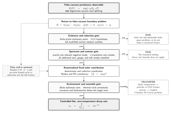
Control map for a flat-space, zero-temperature false-vacuum decay calculation in Euclidean dimensions. The map is schematic, not to scale: the canonical leading bounce returns to the false vacuum, has exactly one relevant negative mode and translational zero modes, and yields a rate only after determinant, renormalization, approximation, and environmental checks pass. If competing thermal saddles or gravitational backreaction are not subleading, the calculation transfers to the corresponding problem. The dotted thin-wall connection is an optional computational aid, not an alternate path to the rate.
Open the control map at full size when reading on a narrow display.
In words, the sequence is: define the false-vacuum persistence observable; solve the correct boundary problem; justify the symmetry and field-space reduction; verify one negative mode and all translation zero modes; form a renormalized prefactor with units of mass to the power ; and only then interpret the result as a rate per spatial volume. A thin-wall formula is an optional approximation inside this sequence, not an independent definition of decay.
Shared comparison. The instanton–bounce boundary and mode comparison contrasts the physical question, endpoint data, zero and negative modes, determinant, and observable for tunneling instantons and decay bounces.
In the dilute regime, well-separated translated copies of the same bounce form approximate multi-bounce configurations. Integrating their centers gives a factor proportional to spacetime volume for each bounce, while division by accounts for indistinguishable copies. Summing over exponentiates the one-bounce contribution. If is the characteristic bounce radius, the dimensionless overlap parameter is parametrically
This condition says that the expected number of events in a bounce-sized Euclidean spacetime region is small Callan and Coleman 1977, pp. 1762–1765.
Scope and failure boundaries
Section titled “Scope and failure boundaries”The construction above assumes a flat, zero-temperature Euclidean functional integral for a canonically normalized scalar and a well-defined false-vacuum state. It does not establish:
- that the displayed solution is the least-action saddle in a multifield, gauge, derivative-coupled, or constrained theory;
- that its Hessian has exactly one relevant negative mode;
- that the determinant and local counterterms have been renormalized consistently;
- that a dilute multi-bounce sum is valid;
- that the Euclidean exponent alone supplies a thermal nucleation rate; or
- that metric backreaction is negligible.
Finite temperature makes Euclidean time periodic and can replace an saddle by a static critical bubble. Curvature makes the metric dynamical and changes both the boundary problem and its negative modes. Those are changes of problem, not small annotations to the flat bounce.
Common pitfalls
Section titled “Common pitfalls”Using instanton endpoints for decay. A decay bounce returns to the same false vacuum at large Euclidean distance. A path connecting two distinct vacua computes a different amplitude and does not acquire a decay interpretation merely because its action is exponential.
Starting exactly at the true vacuum. With zero initial derivative, an exact minimum is a constant solution. A bounce starts nearby, at a center value selected by the false-vacuum asymptotic condition. If the potential admits several bounce branches, compare their actions and spectra rather than assuming that this center value is unique.
Accepting a visually smooth profile. A smooth curve can be an undershoot, a finite-box artifact, or a solution of a restricted ansatz rather than the full equations. Boundary residuals, action stability, mode counting, and box convergence are independent tests.
Exercises
Section titled “Exercises”- Derive the regular expansion .
Solution
Write . Then and . The constant term in the radial equation is
so .
- Let and . Apply the scale variation and show that a stationary bounce satisfies .
Solution
Changing variables to gives
Stationarity at implies
Hence for . This scaling identity is an independent action check for a numerical profile.
- Explain why and is not a false-vacuum bounce boundary condition.
Solution
Those endpoints define a transition amplitude between distinct field configurations. False-vacuum decay is extracted from a false-vacuum persistence amplitude, so the Euclidean configuration must approach at both temporal ends; radial symmetry expresses this as in every direction as .
References
Section titled “References”- Callan, Curtis G., Jr., and Sidney Coleman. “Fate of the False Vacuum. II. First Quantum Corrections.” Physical Review D 16 (1977): 1762–1768. DOI.
- Coleman, Sidney. Aspects of Symmetry: Selected Erice Lectures. Cambridge University Press, 1985, ch. 7, pp. 265–350. DOI.
- Coleman, Sidney. “Fate of the False Vacuum: Semiclassical Theory.” Physical Review D 15 (1977): 2929–2936; erratum, Physical Review D 16 (1977): 1248. DOI.
- Coleman, Sidney, V. Glaser, and André Martin. “Action Minima among Solutions to a Class of Euclidean Scalar Field Equations.” Communications in Mathematical Physics 58 (1978): 211–221. DOI.