Large-Order Growth and the Borel Transform

A perturbative series can diverge at every nonzero coupling and still determine a function asymptotically. For Gevrey-one growth, dividing the coefficient of $g^n$ by $n!$ exposes a Borel-plane function; if that function can be continued with controlled growth along a nonsingular ray, a Laplace integral reconstructs a directional sum. The reconstruction is conditional, not automatic: one must state the coefficient convention, continuation domain, integration direction, and any singularities met on the way.

Required background. Asymptotic scales, remainders, uniformity, and optimal truncation supplies the definition of an asymptotic expansion and remainder estimates. Saddles, control parameters, and loop counting supplies the small parameter and saddle expansion used in the worked integral.

Helpful background. Branches, sheets, analytic continuation, and monodromy explains why analytic continuation and a choice of ray are additional data.

Factorial growth becomes finite-distance analytic structure

Fix the convention, used throughout this chapter,

$$\Phi(g)\sim\sum_{n=0}^{\infty}a_n g^n, \qquad \widehat\Phi(\zeta) =\mathcal B\Phi(\zeta) \equiv\sum_{n=0}^{\infty}\frac{a_n}{\Gamma(n+1)}\zeta^n.$$

If $|a_n|\le C K^n\Gamma(n+1)$, the Borel series converges for $|\zeta|<K^{-1}$. A directional Borel–Laplace sum is

$$\mathcal S_\theta\Phi(g) \equiv \frac1g\int_{0}^{e^{i\theta}\infty} \mathrm d\zeta\,e^{-\zeta/g}\widehat\Phi(\zeta), \qquad \operatorname{Re}\!\left(\frac{e^{i\theta}}g\right)>0.$$

The factor $1/g$ is part of the convention. With it,

$$\frac1g\int_0^{e^{i\theta}\infty} \mathrm d\zeta\,e^{-\zeta/g}\zeta^n =n!\,g^n$$

whenever the ray and $g$ lie in a common convergence sector. Watson’s lemma then recovers the original series as an asymptotic expansion. A uniqueness or reconstruction theorem needs more: analyticity in a sufficiently wide region and a uniform Gevrey remainder bound. The sharp Nevanlinna–Sokal formulation is given by Sokal 1980, Theorem 1, pp. 261–263.

Suppose, near the closest Borel singularity $A\ne0$,

$$\widehat\Phi(\zeta) \sim \frac{C}{(1-\zeta/A)^\beta}.$$

Expanding around the origin gives

$$a_n \sim \frac{C}{\Gamma(\beta)} \frac{\Gamma(n+\beta)}{A^n}.$$

Thus the distance $|A|$ fixes the leading factorial scale, $\arg A$ fixes the coefficient phase or sign pattern, and $\beta$ fixes the power multiplying $n!$. Conversely, late coefficients can estimate a nearby singularity, but they do not by themselves identify it with an instanton, a renormalon, or any other physical mechanism. Multiple singularities of equal modulus interfere, and a conjugate pair produces oscillatory large-order behavior. The contour argument behind this coefficient–singularity relation is developed in Mariño 2015, §3.3, pp. 89–92.

An exact Borel-summable integral

Consider, for $\operatorname{Re}g>0$,

$$F(g)=\int_0^\infty\frac{e^{-t}}{1+gt}\,\mathrm dt.$$

Expanding the denominator before integration gives

$$F(g)\sim\sum_{n=0}^\infty(-1)^n n!\,g^n, \qquad \widehat F(\zeta)=\frac1{1+\zeta}.$$

The series has zero radius of convergence: the ratio of successive term magnitudes is $(n+1)|g|$. Yet its Borel transform is analytic on the positive ray, so

$$\mathcal S_0F(g) =\frac1g\int_0^\infty \frac{e^{-\zeta/g}}{1+\zeta}\,\mathrm d\zeta =\frac{e^{1/g}}g E_1\!\left(\frac1g\right) =F(g).$$

The equality follows by $\zeta=gt$ and is exact, not a numerical fit. At $g=0.1$ it gives $F(g)=0.9156333393979128\ldots$. The least term occurs where $(n+1)g\simeq1$, hence $n_\star\simeq g^{-1}-1$. Stirling’s formula gives a least-term scale proportional to $g^{-1/2}e^{-1/g}$; truncating far beyond $n_\star$ makes the approximation worse. This example separates three notions that are often conflated:

• the power series diverges;
• its optimally truncated partial sums are useful; and
• its Borel transform admits an unobstructed positive-ray Laplace integral that equals the original integral.

None of these facts alone implies that an arbitrary QFT perturbation series is Borel summable.

Borel and transseries map

The figure organizes the chapter’s logic. Read it from the declared series convention to the bounded conclusion, and inspect the status labels below the singularity interpretations: the same Borel singularity can support a theorem in one model, a controlled saddle calculation in another, or only a conjectural correspondence in a harder QFT.

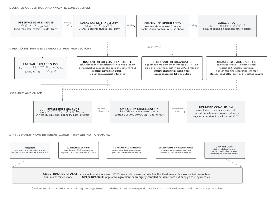
Borel–transseries relations for the convention $\widehat\Phi(\zeta)=\sum a_n\zeta^n/n!$ and $\mathcal S_\theta=g^{-1}\int e^{-\zeta/g}\widehat\Phi\,\mathrm d\zeta$. Solid arrows are analytic deductions, dashed arrows require model-specific saddle or momentum-region input, and the terminal consistency check is not a proof that all sectors of a QFT have been found. The diagram is schematic and not to scale.

The nonvisual reading is:

1. a declared observable and coefficient convention determine a formal series;
2. Gevrey-one bounds make the local Borel transform analytic near the origin;
3. continued Borel singularities determine directional ambiguities and large-order scales;
4. an instanton, renormalon, or quasi-zero-mode interpretation needs independent model-specific evidence;
5. equations, boundary data, or an integration cycle determine which exponential and logarithmic sectors may occur and fix their transseries parameters;
6. opposite lateral ambiguities must cancel in a well-defined real observable when the relevant sectors are present; and
7. cancellation is a stringent consistency condition, not a construction or completeness theorem.

Shared comparison. The exact and rigorous status comparison distinguishes exact-model reconstruction, constructive theorems, controlled calculations, and open limits.

What the transform does not decide

A Borel transform reorganizes coefficient data. It does not generate the perturbative coefficients, prove the required analytic continuation, select a physical contour, or determine boundary conditions. A singularity on the Laplace ray makes the ordinary directional sum ambiguous; the next page derives the two lateral sums. General Écalle theory supplies a much richer algebra of singularities and sector relations, but that theory is beyond this page’s scope.

For QFT, the observable, regulator, renormalization scheme, and order of limits must remain fixed while coefficients are compared. A finite-dimensional integral can prove the mechanism exists without establishing it for a renormalized infinite-volume field theory. The handoff to evidence and limits for resurgence in QFT makes that inference boundary explicit.

Common pitfalls

Divergent does not mean meaningless. An asymptotic series can approximate a function extremely well up to its least term. The remainder, rather than convergence of partial sums as the order tends to infinity, is the relevant criterion.

Alternating does not by itself prove Borel summability. The sign pattern suggests where a leading singularity may lie, but analytic continuation and exponential-growth bounds along the entire Laplace ray still have to be established.

A Borel singularity is not automatically an instanton. The coefficient data locate analytic structure. A saddle interpretation requires a specified complexified action, integration cycle, fluctuation factor, and matching normalization.

Exercises

1. For $a_n=(-1)^n\Gamma(n+\beta)/\Gamma(\beta)$ with $\operatorname{Re}\beta>0$, compute $\widehat\Phi(\zeta)$ and locate its nearest singularity.

Solution

The generalized binomial series gives

$$\widehat\Phi(\zeta) =\sum_{n\ge0}\frac{(-1)^n(\beta)_n}{n!}\zeta^n =(1+\zeta)^{-\beta}.$$

Its nearest singularity is at $\zeta=-1$. For noninteger $\beta$ it is a branch point; for positive integer $\beta$ it is a pole of order $\beta$.

2. Show directly that the optimally truncated term of $\sum(-1)^n n!g^n$ has exponential scale $e^{-1/g}$ for small positive $g$.

Solution

The term ratio is $(n+1)g$, so the minimum occurs at $n\simeq g^{-1}$. Stirling’s formula gives

$$n!g^n\sim\sqrt{2\pi n}\left(\frac{ng}{e}\right)^n \sim\sqrt{\frac{2\pi}{g}}e^{-1/g}.$$

The algebraic prefactor depends on the precise integer chosen, but the exponential scale is fixed.

References

• Mariño, Marcos. Instantons and Large N: An Introduction to Non-Perturbative Methods in Quantum Field Theory. Cambridge University Press, 2015. doi:10.1017/CBO9781107705968.
• Sokal, Alan D. “An Improvement of Watson’s Theorem on Borel Summability.” Journal of Mathematical Physics 21 (1980): 261–263. doi:10.1063/1.524408.