What Does Nonperturbative Mean?

A statement is nonperturbative only relative to a specified expansion or formulation. An effect proportional to $e^{-A/g}$ is invisible to every power of $g$ near $g=0$; a large-$N$ saddle reorganizes rather than completes the coupling expansion; a regulated numerical calculation can include contributions absent from diagrammatic perturbation theory but is controlled only after its regulator, limits, and errors are tested. The operative questions are therefore: nonperturbative in what variable, for which observable, in which order of limits, and with what check?

Required background. Asymptotic scales, remainders, and optimal truncation supplies the distinction between a formal series and its remainder. Regulators, cutoffs, and continuum limits supplies the limit that turns a regulated calculation into a statement about a continuum theory.

Helpful background. Saddles and the semiclassical expansion explains the local Gaussian construction, while effective field theory as a controlled expansion explains errors organized by ratios of physical scales.

Nonperturbative relative to what?

Let an observable $\mathcal O(g)$ have a formal expansion about $g=0$,

$$\mathcal O(g)\sim\sum_{n=0}^{\infty}a_n g^n.$$

A contribution $\delta\mathcal O(g)$ is beyond all orders in this expansion if, for every fixed integer $N\geq 0$,

$$\lim_{g\to0^+}\frac{\delta\mathcal O(g)}{g^N}=0.$$

The standard example is $\delta\mathcal O(g)=C(g)e^{-A/g}$ with $A>0$ and $C(g)$ at most algebraic near the origin. Every derivative of the pure exponential vanishes at $g=0$ after continuous extension, so its Taylor series is identically zero even though the function is not. This is a precise sense in which a saddle sector can be nonperturbative.

That definition is not exhaustive. A quantity may also be called nonperturbative because the calculation does not expand in the microscopic coupling at all—for example, a continuum-extrapolated lattice correlation function. In that case the word describes the formulation, not a proof of accuracy. Conversely, a large value of a coupling says that a particular weak-coupling expansion is unavailable; it does not say that every reorganization is uncontrolled.

The relation among comparison, calculation, and conclusion is summarized below. Inspect the separate control test: the method name alone never supplies it.

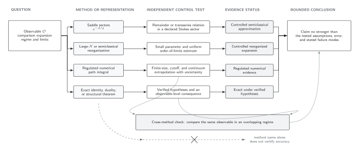
“Nonperturbative” specifies what a contribution or formulation is not expanded in. Reliability comes from an independent remainder, small parameter, exact hypothesis, continuum limit, or validation test; the diagram is schematic and not a ranking of methods.

Double-well splitting beyond a local series

Consider a particle of mass $m$ in a symmetric potential $V(q)=\lambda(q^2-a^2)^2$. Perturbation theory about either minimum begins from the same harmonic frequency,

$$\omega^2=\frac{V''(a)}{m}=\frac{8\lambda a^2}{m},$$

and generates one formal local energy series. It cannot distinguish the even and odd combinations of wavefunctions supported near the two wells. The distinction is global: a Euclidean trajectory crosses the barrier with action

$$S_0=\int_{-a}^{a}\!\mathrm dq\,\sqrt{2mV(q)} =\frac{4}{3}a^3\sqrt{2m\lambda}.$$

In the semiclassical regime $S_0/\hbar\gg1$, the two lowest energies have the structure

$$E_\pm=E_{\mathrm{loc}}\mp K e^{-S_0/\hbar} \left[1+O\!\left(\frac{\hbar}{S_0}\right)\right],$$

where $K$ is fixed by the fluctuation determinant and collective-coordinate normalization. The splitting $\Delta E=2Ke^{-S_0/\hbar}+\cdots$ is smaller than every power of $\hbar$ and therefore absent from the perturbative series about one minimum. Coleman derives the dilute-instanton construction and its determinant logic in Coleman 1985, ch. 7, § 2.2, pp. 270–277; Mariño gives a modern calculation in Mariño 2015, ch. 1, §§ 1.8–1.9, pp. 38–53.

This example also identifies the control parameter and its failure. The exponential hierarchy is useful when $S_0/\hbar$ is large and instantons are well separated. A numerically small answer obtained where the saddle gas overlaps is not thereby controlled.

Four distinct routes beyond one power series

The same adjective covers calculations with different logical structures.

1. Additional saddle sectors. Terms such as $e^{-S_0/\hbar}$ or $e^{-8\pi^2/g^2}$ lie beyond the chosen loop series. Control requires the saddle action, fluctuation spectrum, measure, integration cycle, and interactions among saddles.
2. Reorganized limits. A $1/N$ expansion can be useful at fixed ’t Hooft coupling even when a small-coupling expansion is not. Its error is a power of $1/N$, possibly nonuniform near a phase transition; it is not automatically an exact finite-$N$ answer. The original diagrammatic scaling is established in ’t Hooft 1974, pp. 461–473.
3. Exact special structures. Integrability, localization, topology, or symmetry protection may determine a selected observable under stringent hypotheses. Exactness of that object does not imply that the whole theory, every deformation, or every real-time observable is solved.
4. Regulated definitions and computation. A lattice or Hamiltonian regulator can retain effects missed by a weak-coupling expansion. Reliability then depends on finite-volume, discretization, statistical, algorithmic, and continuum-limit tests. Wilson’s gauge-invariant lattice construction is a canonical example of a formulation rather than an error certificate Wilson 1974, §§ II–IV, pp. 2448–2456.

Resummation of a divergent perturbative series deserves separate wording. Borel or other summation can recover information not visible at finite order, but a resummed perturbative sector may still carry ambiguities or require additional transseries data. Those questions are developed in Resurgence and Transseries.

A claim must carry its control data

The following semantic table is a reusable test. “Status class” describes the support for the stated result, not the prestige of a method.

Claims, controls, errors, and falsifiers for representative nonperturbative methods

Claim	Model	Observable	Regime	Control parameter or hypothesis	Status class	Error form	Falsifier	Continue with
The lowest double-well levels split by 2K e−S₀/ℏ at leading order	Symmetric quartic double well	Level splitting ΔE	S₀/ℏ ≫ 1	Dilute saddles and a positive one-instanton determinant ratio	Controlled semiclassical approximation	Relative corrections in ℏ/S₀ and saddle overlap	Exact diagonalization disagrees as S₀/ℏ grows	Instanton tunnel splitting
Planar diagrams dominate a normalized single-trace sector	Matrix or gauge theory with declared large-N scaling	Connected correlator	Fixed ’t Hooft coupling away from nonuniform limits	1/N counting and observable normalization	Controlled reorganized expansion	Powers of 1/N with possible nonuniform enhancement	Index counting or finite-N data violate the predicted scaling	Large-N normalizations
A factorized S matrix satisfies a proposed exact bootstrap	Specified integrable 1+1-dimensional QFT	Two-body S(θ)	Stable spectrum and factorized scattering	Unitarity, crossing, Yang–Baxter consistency, pole and completeness assumptions	Exact conditional construction	CDD and completeness ambiguity	Spectrum, residue, locality, or finite-volume checks fail	Exact S-matrix bootstrap
A regulated mass approaches a continuum value	Declared lattice action and universality class	Mass gap	Controlled volume and lattice-spacing sequence	a → 0, L → ∞, scale setting, and fit stability	Regulated numerical evidence	Statistical plus continuum and volume systematics	Alternative discretizations do not converge to the same limit	Lattice continuum inference
A nontrivial anomaly excludes a unique symmetric trivial gapped infrared state	QFT with specified symmetry and background fields	Infrared realization class	Symmetry preserved along the flow	Nontrivial anomaly modulo local counterterms	Exact obstruction under hypotheses	No approximation error; only hypothesis and classification scope	A symmetric trivial gapped realization reproduces the background response	Anomaly constraints

A practical decision test

Before accepting a nonperturbative statement, record:

1. the observable and its normalization;
2. the comparison expansion or regulated formulation;
3. the parameter, theorem hypotheses, or convergence test that controls the method;
4. the order of regulator, volume, source, and asymptotic limits;
5. one independent check or solvable limit; and
6. a condition under which the claim would fail.

Two calculations that share the same ansatz, effective action, or calibration data are not fully independent evidence. Likewise, agreement with one number does not validate quantities that probe different analytic continuation, topology, or infrared limits.

Common pitfalls

Equating nonperturbative with numerical. Numerical work may evaluate either perturbative coefficients or a regulated formulation containing all sectors. Its reliability is determined by convergence and uncertainty tests, not by the presence of a computer.

Equating strong coupling with lack of control. Strong coupling invalidates a nominated weak-coupling series. A dual weakly coupled description, large-$N$ limit, exact theorem, or regulated continuum extrapolation may still provide control, but each has a different error statement.

Calling an exponentially small term negligible. A term beyond all orders can be the leading effect for a symmetry-forbidden splitting, decay width, or ambiguity cancellation. Smallness and physical importance are separate questions.

Exercises

For $f(g)=e^{-1/g}$ at $g>0$, extended by $f(0)=0$, show that $f(g)=o(g^N)$ for every fixed $N$. Explain why a zero Taylor series does not imply a zero function.

Solution

Set $x=1/g$. Then $f(g)/g^N=x^N e^{-x}\to0$ as $x\to\infty$, because the exponential dominates every polynomial. All right derivatives at the origin vanish, so the Taylor series is zero, while $f(g)>0$ for every $g>0$. Analyticity, not smoothness alone, would be needed to reconstruct the function from that series.

A calculation reports a continuum-extrapolated number at three lattice spacings but only one spatial volume. Which word in “nonperturbative determination” is justified, and which control claim remains unsupported?

Solution

“Nonperturbative” may correctly describe the regulated formulation if it does not expand in the coupling. “Determination” is not yet justified for the infinite-volume observable: the volume dependence has not been bounded. The lattice-spacing extrapolation and thermodynamic-limit test are distinct.

References

• Coleman, Sidney. Aspects of Symmetry: Selected Erice Lectures. Cambridge University Press, 1985, ch. 7, § 2.2, pp. 270–277. DOI.
• Mariño, Marcos. Instantons and Large N: An Introduction to Non-Perturbative Methods in Quantum Field Theory. Cambridge University Press, 2015, ch. 1, §§ 1.8–1.9, pp. 38–53. DOI.
• ’t Hooft, Gerard. “A Planar Diagram Theory for Strong Interactions.” Nuclear Physics B 72 (1974): 461–473. DOI.
• Wilson, Kenneth G. “Confinement of Quarks.” Physical Review D 10 (1974): 2445–2459. DOI.