Schwinger–Dyson Hierarchies and Renormalization Inputs

Schwinger–Dyson equations are exact consequences of integration by parts in the regulated functional integral. Repeated differentiation turns one identity into an infinite hierarchy relating an $n$-point function to higher functions. Exactness ends there: a finite calculation must declare a regulator, counterterms and renormalization conditions, boundary or asymptotic data, a closure, a solution branch, and tests of physical admissibility such as positivity. An algebraically self-consistent propagator without those inputs is not yet a solution of the QFT.

Required background. Schwinger–Dyson identities supplies the functional integration-by-parts identity, while the 1PI effective action supplies proper vertices. Helpful background. Renormalization conditions, schemes, and finite parts supplies the counterterm inputs.

From one exact identity to a hierarchy

For a regulated Euclidean scalar integral with source $J$,

$$Z[J] =\int\mathcal D\phi\, \exp\!\left[ -S_E[\phi]+\int J\phi \right],$$

translation invariance of the measure gives

$$0 =\int\mathcal D\phi\, \frac{\delta}{\delta\phi(x)} \exp\!\left[ -S_E[\phi]+\int J\phi \right].$$

Therefore

$$\left\langle \frac{\delta S_E}{\delta\phi(x)} \right\rangle_J =J(x).$$

Differentiating with respect to $J$ inserts fields and generates equations for connected correlators. Legendre transforming instead writes the same hierarchy in terms of the mean field, full propagator, and proper vertices. These identities are exact for the regulated measure and its boundary conditions; an anomalous Jacobian or a regulator that breaks a symmetry contributes an extra term rather than disappearing.

Schwinger’s source formulation and Dyson’s propagator reorganization supply the historical foundations Schwinger 1951, pp. 452–455, Dyson 1949, §§ 3–5.

A renormalized scalar two-point equation

Take

$$S_E =\int\mathrm d^d x\, \left[ \frac{Z_\phi}{2}(\partial_\mu\phi)^2 +\frac{m_R^2+\delta m^2}{2}\phi^2 +\frac{\lambda_R+\delta\lambda}{4!}\phi^4 \right]$$

in a $\mathbb Z_2$-symmetric phase with $\langle\phi\rangle=0$. Differentiating the exact identity once and then setting $J=0$ gives

$$\begin{aligned} \delta(x-y) ={}& \left[ -Z_\phi\partial_x^2 +m_R^2+\delta m^2 \right]G(x,y) \\ &+\frac{\lambda_R+\delta\lambda}{3!} \left\langle \phi^3(x)\phi(y) \right\rangle . \end{aligned}$$

The four-field expectation decomposes as

$$\left\langle \phi^3(x)\phi(y) \right\rangle =3G(x,x)G(x,y) +G_c^{(4)}(x,x,x,y).$$

For a translation-invariant regulator, Fourier transformation yields

$$G^{-1}(p) =Z_\phi p^2+m_R^2+\delta m^2 +\frac{\lambda_R+\delta\lambda}{2} \int_q G(q) +\Sigma_4(p),$$

where $\int_q$ includes the declared regulator and $\Sigma_4(p)G(p)$ is defined by the Fourier transform of $(\lambda_R+\delta\lambda)G_c^{(4)}(x,x,x,y)/3!$. The equation for $G$ therefore requires the connected four-point function, whose equation requires higher functions. Replacing $\Sigma_4$ by zero, a vertex ansatz, or a skeleton subset is a closure, not part of the exact identity.

Counterterms are fixed only after renormalization conditions are stated. A momentum-subtraction example is

$$\left. \Gamma_R^{(2)}(p) \right|_{p^2=\mu^2} =\mu^2+m_R^2, \qquad \left. \frac{\partial\Gamma_R^{(2)}}{\partial p^2} \right|_{p^2=\mu^2} =1,$$

and

$$\left. \Gamma_R^{(4)}(p_1,p_2,p_3,p_4) \right|_{\mathrm{sym},\,\mu} =\lambda_R.$$

Changing these finite conditions changes intermediate dressings and parameters. A physical prediction must be translated between schemes or expressed through a scheme-independent observable.

Inputs that select a physical solution

The hierarchy and renormalization conditions can still admit multiple branches. A complete problem also specifies:

• the regulator and how it is removed;
• the counterterm basis and all finite renormalization conditions;
• spacetime, volume, temperature, boundary conditions, and vacuum sector;
• ultraviolet asymptotics and any infrared regularity conditions;
• reality, symmetry, crossing, and spectral constraints appropriate to the operator;
• the branch-continuation rule as parameters are varied.

For a physical neutral scalar in a positive-metric theory, a Euclidean two-point function may admit

$$G(p_E^2) =\int_0^\infty\mathrm ds\, \frac{\rho(s)}{p_E^2+s}, \qquad \rho(s)\ge0.$$

Reflection positivity and the ultraviolet normalization then constrain candidate solutions. Gauge-fixed elementary fields need not satisfy this scalar positivity test; the observable and state space must be declared before applying it. The reconstruction assumptions and the role of reflection positivity are stated in Osterwalder and Schrader 1973, pp. 86–94.

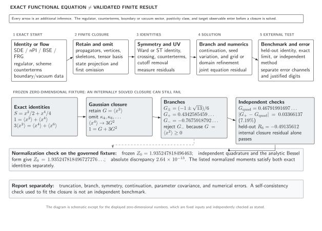
Functional-equation closure and validation map

The diagram separates the exact identity from every later inference. The lower row is a frozen zero-dimensional benchmark: it makes the retained moment, omitted cumulants, branch rejection, exact residual, and external quadrature discrepancy visible.

Exact functional equations do not certify a finite solution. Every closure must list retained and omitted structures, preserve the declared renormalization and symmetry conditions, identify the selected branch, pass numerical residual tests, and face an independent benchmark with separately reported errors. In the schematic zero-dimensional example, the negative Gaussian root is rejected because $\langle x^2\rangle$ cannot be negative; the positive root satisfies the closed equation but differs from exact quadrature.

Frozen zero-dimensional fixture

Let

$$Z_0 =\int_{-\infty}^{\infty}\mathrm dx\, e^{-x^2/2-x^4/4}.$$

Integration by parts gives the exact identities

$$1=\langle x^2\rangle+\langle x^4\rangle, \qquad 3\langle x^2\rangle =\langle x^4\rangle+\langle x^6\rangle.$$

The governed fixture records

$$\begin{aligned} Z_0^{\mathrm{frozen}}&=1.935247818496463,\\ \langle x^2\rangle&=0.4679199169736715,\\ \langle x^4\rangle&=0.5320800830263535,\\ \langle x^6\rangle&=0.8716796678946697. \end{aligned}$$

The normalized moments satisfy both identities to the shown precision. Independent 80-digit quadrature and the analytic Bessel representation give

$$Z_0^{\mathrm{check}} =1.935247818496727276425839913\ldots,$$

which differs from the frozen normalization by $2.64\times10^{-13}$. The frozen value is therefore reproduced only to that absolute tolerance; its final displayed digits are not independently validated. The discrepancy does not affect the separately normalized moments at the precision quoted.

A Gaussian closure retains $G=\langle x^2\rangle$ and sets the connected fourth cumulant to zero:

$$\langle x^4\rangle\longmapsto3G^2.$$

The first exact identity becomes

$$1=G+3G^2, \qquad G_\pm=\frac{-1\pm\sqrt{13}}{6}.$$

Positivity rejects $G_-=-0.7675918792\ldots$. The accepted closed branch gives

$$G_+=0.4342585459\ldots,$$

which differs from exact quadrature by $0.0336613711\ldots$, or $7.19\%$. Moreover, also imposing the Gaussian sixth moment $\langle x^6\rangle=15G^3$ leaves the second-identity residual

$$R_6 =3G-(3G^2+15G^3) =-0.4913561224\ldots.$$

Internal solution of the first closed equation is therefore not external validation.

Functional-method validation comparison

The table is the semantic counterpart to the diagram. It records the minimum information needed before digits from a finite functional calculation can be interpreted.

Required validation record for representative continuum functional methods.

Method	Exact identity and external inputs	Ansatz, projection, and omitted structures	Branch and symmetry residuals	Solver and truncation checks	Independent benchmark and covariance	Justified reporting
Schwinger–Dyson hierarchy	Regulated integration-by-parts identity; counterterms, renormalization conditions, boundary data, and operator positivity class	Retained propagators and vertices; tensor basis and every omitted higher function	Parameter continuation and competing solutions; Ward or Slavnov–Taylor residuals and ultraviolet asymptotics	Equation residual, grid and cutoff refinement, initial-condition dependence, and nested closure spread	Exact limit, perturbative coefficient, quadrature or lattice observable; propagate shared parameter and vertex covariance	Separate truncation, branch, symmetry, parameter, continuation, and numerical errors; round only after their combined scale is known
2PI or nPI stationarity	Declared Legendre transform, regulator, counterterms, and stationary equations	Skeleton loop order and variational vertices; omitted skeletons and crossing channels	Chosen stationary point; global, Ward, and conservation residuals	Stationarity norm, discretization, loop-order variation, and double-counting check	Perturbative expansion, exactly solvable limit, or another regulator; retain covariance between self-energy and derived kernel	Do not quote more digits than the larger of truncation spread and benchmark discrepancy supports
Bethe–Salpeter or Faddeev equation	Four- or six-point pole equation; constituent renormalization and analytic domain	Kernel construction, momentum partition, tensor basis, and omitted crossed or many-body kernels	Eigenvalue branch and state quantum numbers; vector or axial Ward-identity residual	Eigenpair residual, basis and contour refinement, normalization, and kernel variation	Derive the kernel from the same self-energy as an internal check; compare an independent spectrum or controlled threshold; propagate constituent–kernel covariance	A Euclidean eigenvalue is not a physical pole until analytic continuation and singularity access are controlled
Functional RG projection	Exact regulated flow plus ultraviolet action and infrared limit	Operator basis, field expansion, projection momenta, and omitted momentum dependence	Fixed-point or phase branch; modified Ward-identity residuals	Integrator residual, regulator family, projection point, field order, and derivative-order variation	Perturbative coefficients, large-N or exact limits, Monte Carlo or bootstrap data; retain covariance of fitted couplings	Critical digits require a visible convergence pattern, not one stable regulator choice
Spectral or complex-momentum reconstruction	Euclidean data plus a stated spectral representation, analyticity domain, asymptotics, and subtraction terms	Basis or prior for the spectral density, contour choice, and unresolved poles or cuts	Continuation branch; sum-rule, reality, and positivity tests where applicable	Data perturbation, basis and regularization variation, mock-data recovery, and complex-plane residual	Known spectral model, real-time calculation, or independent scattering data; publish data covariance	Underdetermined features are bounds or prior-dependent reconstructions, not unique spectral facts
Gauge-fixed coupled system	Gauge-fixed functional identities, BRST or Slavnov–Taylor inputs, renormalization point, and Gribov prescription	Propagator–vertex tensor basis, ghost sector, kernel matching, and omitted gauge-completion terms	Infrared branch and copy sensitivity; identity residuals at representative momenta	Coupled residuals, grid and volume checks, initial branches, and coordinated ansatz variation	Gauge-invariant observable, lattice calculation in the same gauge, or perturbative ultraviolet result; propagate shared-input covariance	Gauge-fixed positivity violation alone is not a gauge-invariant confinement conclusion

Common pitfalls

Calling the hierarchy a solution. The exact hierarchy is infinite. A finite result begins only after omitted functions and closure assumptions are named.

Renormalizing after truncation without checking consistency. Counterterms and vertex relations can be linked by symmetry. A subtraction that makes one equation finite can still leave another identity inconsistent.

Selecting a branch by solver convergence. Iteration converges to a basin of attraction, not necessarily the physical branch. Continuity, positivity, symmetry, free-energy, or external data must provide the selection criterion.

Exercises

1. Reproduce the two scalar identities by integrating the derivatives of $x e^{-S(x)}$ and $x^3e^{-S(x)}$, where $S=x^2/2+x^4/4$.

Solution

Boundary terms vanish because $e^{-S}$ decays faster than any power. Thus

$$0 =\int\mathrm dx\, \frac{\mathrm d}{\mathrm dx} \left(xe^{-S}\right) =Z_0 \left[ 1-\langle xS'(x)\rangle \right],$$

so $1=\langle x^2\rangle+\langle x^4\rangle$. Likewise,

$$0 =\int\mathrm dx\, \frac{\mathrm d}{\mathrm dx} \left(x^3e^{-S}\right) =Z_0 \left[ 3\langle x^2\rangle -\langle x^3S'(x)\rangle \right],$$

which gives $3\langle x^2\rangle=\langle x^4\rangle+\langle x^6\rangle$.

2. Explain why $G_+$ passing the first closed equation does not make its $7.19\%$ error a numerical error.

Solution

The algebraic equation can be solved to arbitrary numerical precision, so its solver residual can be essentially zero. The difference from exact quadrature comes from replacing the true fourth moment by $3G^2$ and omitting connected cumulants. It is truncation error. The nonzero second-identity residual provides a diagnostic not used to determine $G_+$.

Continue

Closure, Symmetry Constraints, and Branch Selection turns the map into a practical closure record. Functional-Method Validation and Error Control separates the error channels and connects them to independent evidence.

References

• Dyson, Freeman J. “The S Matrix in Quantum Electrodynamics.” Physical Review 75 (1949): 1736–1755. DOI.
• Osterwalder, Konrad, and Robert Schrader. “Axioms for Euclidean Green’s Functions.” Communications in Mathematical Physics 31 (1973): 83–112. DOI.
• Schwinger, Julian. “On Green’s Functions of Quantized Fields. I.” Proceedings of the National Academy of Sciences 37 (1951): 452–455. DOI.