

Renormalization Conditions, Schemes, and Finite Parts
A renormalization scheme is a coordinate system on the same family of renormalized theories. The divergent local terms fix which counterterms are required; renormalization conditions fix their finite parts and thereby define the numerical mass, coupling, and field normalization called “renormalized.” Minimal subtraction, momentum subtraction, on-shell conditions, and physical input schemes generally assign different numbers to those coordinates.
They describe the same physics only after a finite parameter and field map is applied. Comparing an MS̄ coupling directly with a momentum-subtraction coupling at the same numerical value compares different theories. The valid check is to match the same inputs, translate the coordinates to the calculated order, and compare a non-input prediction; the difference should begin one order beyond the truncation.
Required background. Dimensional Regularization and Minimal Subtraction fixes the modified-MS pole convention used below.
Helpful background. The 1PI Effective Action and Mean-Field Equations supplies the inverse two-point and proper-vertex language. Local Counterterms and Subdivergence Structure explains why two local schemes can differ only by finite local terms.
Finite conditions define the renormalized coordinates
Section titled “Finite conditions define the renormalized coordinates”Let a regulated bare parameter be written in scheme as
The same bare theory can be parameterized in scheme :
Equating the two expressions and removing the regulator gives a finite map,
Fields can also require a finite map,
The coefficients depend on the two scheme definitions. They are not additional observables. Once the map is fixed, an exact observable has the same value in both coordinate systems.
At finite order, suppose
Inverting the map and substituting gives
Thus . The coefficient of a truncated expansion changes precisely enough to compensate the changed coupling. Scheme independence never means equality of the intermediate coefficients.
Collins formulates a change of renormalization prescription as a finite reparametrization of couplings, masses, and fields and proves equality of the corresponding physics Collins 1984/2023, § 7.1, pp. 169–176.
Four common choices
Section titled “Four common choices”| Scheme type | Defining condition | Main advantage | Main caution |
|---|---|---|---|
| MS or MS̄ | Subtract only the declared dimensional poles, with or without the standard package | Mass independent; exposes renormalization-group structure | Parameters are not direct observables; heavy fields do not decouple automatically |
| Momentum subtraction | Fix inverse propagators and vertices at specified nonexceptional Euclidean momenta | Kinematic meaning is explicit; useful for nonperturbative comparisons | Generally mass and gauge-parameter dependent; exceptional points can create infrared problems |
| On shell | Put a stable-particle pole at its physical mass and normalize its residue; define charges from a stated physical limit | Inputs are closely tied to measured quantities | Infrared singularities, confinement, massless particles, and unstable states can obstruct naive conditions |
| Physical or observable based | Define parameters from a complete set of measured infrared-safe observables | Gauge invariant when the observables are | Often process specific; translations may contain large logarithms |
MS and MS̄ differ only by a conventional finite rescaling of , but writing “MS” while using the modified pole package creates a finite mismatch. Collins treats mass-shell oversubtractions and minimal subtraction separately, making clear that the difference is a finite prescription choice after locality is secured Collins 1984/2023, §§ 5.9–5.11, pp. 130–137.
On-shell two-point conditions
Section titled “On-shell two-point conditions”For a stable scalar with Minkowski inverse propagator
unit pole residue is imposed by
These conditions fix the finite mass and field counterterms. For an unstable particle the invariant object is instead a complex pole; imposing a real-axis residue condition can be gauge dependent and physically misleading. Confining fields have no asymptotic one-particle pole at all.
Nonexceptional momentum subtraction
Section titled “Nonexceptional momentum subtraction”For a Euclidean scalar theory, a MOM scheme can impose
At the symmetric four-point configuration,
Keeping every channel nonzero avoids an artificial infrared singularity in a massless limit. The numerical value of an off-shell MOM parameter can depend on the gauge and projector; only a translated physical prediction is a gauge-invariant checkpoint. Gauge-parameter dependence of off-shell counterterms and its cancellation in physical quantities is developed in Collins 1984/2023, § 12.4, pp. 309–314.
One-loop MS̄-to-MOM map in scalar φ⁴ theory
Section titled “One-loop MS̄-to-MOM map in scalar φ⁴ theory”Use the Euclidean -invariant scalar theory and the convention of the previous pages. Factor the common from the proper four-point coefficient. In MS̄,
where
To isolate the coupling map, take the mass to be matched by the same finite input condition in both descriptions. A one-loop difference in the mass coordinate inserted inside would first change the displayed coupling map at the next order.
Define by demanding that the proper vertex at the symmetric point equal the tree coefficient:
Evaluating the MS̄ expression at that point gives the finite map
Its inverse is
Substituting into the MS̄ vertex yields
At the subtraction point the bracket vanishes, as the MOM definition requires. Away from that point, this is the same one-loop proper vertex as the MS̄ expression, written in different coordinates. The local finite term moved into the definition of the coupling; the nonlocal differences remain in the prediction.
After analytic continuation, the same equality holds for the one-loop scalar scattering amplitude. At this order scalar theory has no field-strength correction, so no additional external residue enters. Both schemes therefore predict the same channel logarithms and cuts through ; their difference begins at .
What the bare-to-observable map requires
Section titled “What the bare-to-observable map requires”Calculations A and B can use different counterterms and renormalized coordinates. Their dashed paths impose the same finite input and normalization conditions; any finite scheme translation is completed before the solid output paths reach the comparison.
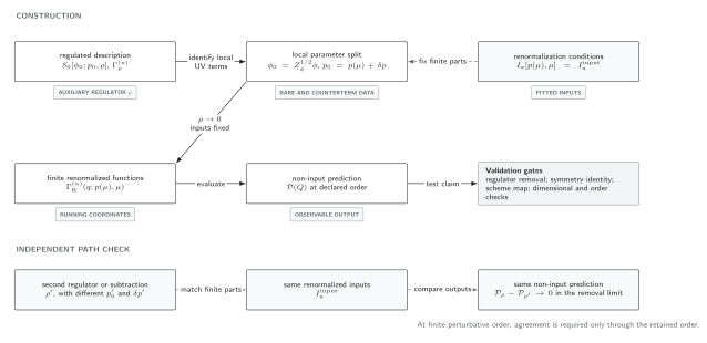
Regulator removal compares a non-input quantity at the same kinematics and retained order. A change of subtraction convention is a coordinate translation within this comparison, not a third regulator. Locality and the same restored symmetry identities remain necessary. The map is schematic; orderwise agreement is not a nonperturbative continuum construction.
The common regulator-comparison fields specialize to a finite scheme comparison as follows:
| Item | Scheme A | Scheme B | Equality test |
|---|---|---|---|
| Regulator convention | Same or explicitly translated | Same or explicitly translated | No hidden change in , , or normalization |
| Renormalized inputs | Declared observables or conditions | The same physical information | Equal input values after translation |
| Finite map | Bare relations agree through the retained order | ||
| Symmetry identity | Restored with scheme-A finite terms | Restored with scheme-B finite terms | Same Ward or Slavnov–Taylor identity |
| Non-input quantity | after an order- calculation | ||
| Residual variation | Change of , subtraction point, or allowed finite terms | Corresponding translated change | Used as a diagnostic, not a universal probability distribution |
For the scalar benchmark, the map above is exact through one loop at the stated kinematics. A reproducible calculation should cover evaluating , applying the forward and inverse maps, and checking the round-trip residual.
Scheme choice and perturbative truncation
Section titled “Scheme choice and perturbative truncation”An exact prediction is scheme independent, but a truncated result retains higher-order scheme dependence. This has three practical consequences.
First, apply a scheme map to the same order as the calculation. Using a two-loop amplitude with only a tree-level parameter identification leaves a spurious one-loop mismatch.
Second, choose scales and schemes that do not manufacture large coefficients. A MOM point far from all physical scales or a physical input containing a large hierarchy can move a large logarithm into the finite map rather than eliminate it.
Third, scheme variation is a useful stress test but not, by itself, a statistically calibrated uncertainty. A small variation can miss a large next coefficient, while an extreme finite redefinition can exaggerate the remainder. Combine it with scale variation, known asymptotics, power counting, and benchmark comparisons appropriate to the problem.
Heavy-particle thresholds add another qualification. A mass-independent scheme retains heavy fields in the beta functions until an effective theory is matched across the threshold. That is not a failure of MS̄; it is a signal that running and matching are separate operations, developed later in this volume.
Common pitfalls
Section titled “Common pitfalls”Setting two scheme couplings to the same number. Their equality is not the matching condition. Use the finite map derived from a common bare theory or common physical inputs.
Changing the scheme in the loop term but not the tree term. Re-expand the entire truncated prediction, including masses, fields, and external residues.
Subtracting at exceptional momentum in a massless theory. Zero momentum can turn a ultraviolet definition into an infrared singular one. Use a nonexceptional Euclidean point or an explicitly infrared-safe prescription.
Treating an off-shell MOM coupling as gauge invariant. It can depend on gauge fixing and projectors. Translate it into a physical observable before making an invariant claim.
Using a real on-shell condition for an unstable state. The stable-pole assumptions fail. Use the complex pole and a treatment appropriate to unstable particles.
Reading scheme variation as a confidence interval. It samples selected higher-order terms but has no universal probabilistic interpretation.
Exercises
Section titled “Exercises”1. Invert the scalar map. Verify the inverse relation through .
Solution
Write , with . Iterative inversion gives . Substituting it into the forward map leaves .
2. Check the MOM condition. Set all three channel invariants to in the MOM vertex.
Solution
The one-loop bracket becomes , so , exactly as defined.
3. Diagnose a comparison. Two calculations use the same numerical coupling, one in MS̄ and one in MOM, and differ at order . Is this scheme dependence of a physical prediction?
Solution
Not yet. The same number labels different theories in the two schemes. Apply the finite map or fit both couplings to the same input first. Any remaining difference should then start at order .
Finite-coordinate result
Section titled “Finite-coordinate result”A scheme change moves finite local terms between parameters and coefficient functions:
MS̄, MOM, on-shell, and physical schemes are therefore tools with different conditioning and bookkeeping properties, not competing physical laws.
Continue to Regulator Removal and Renormalized Predictions to combine finite matching with the removal limit, symmetry checks, and an explicit remainder. Continue later to threshold matching for the separate question of changing active degrees of freedom.
References
Section titled “References”- Collins, John C. 1984; open-access reissue 2023. Renormalization: An Introduction to Renormalization, the Renormalization Group and the Operator-Product Expansion. Cambridge Monographs on Mathematical Physics. Cambridge University Press. DOI and Open PDF.