

Effective Field Theory as a Controlled Expansion
An effective field theory is controlled when its error can be reduced systematically by adding the next terms required by a declared expansion. The ultraviolet completion may be known, partly known, or entirely unknown; predictivity instead rests on a domain, active degrees of freedom, symmetry, power counting, and a finite set of coefficients at each target accuracy. This page tests that control using the exact tree-level heavy-exchange contribution in a stable scalar model, keeping its contribution-relative truncation error distinct from the error of the total amplitude.
Required background. Regulator Removal and Renormalized Predictions supplies the distinction between a regulator and a physical prediction, while Local and Composite Operator Insertions supplies the local-operator grammar. Helpful background. Free-Field OPE Preview previews how short-distance effects can be organized by local operators.
A finite prediction from an infinite action
Section titled “A finite prediction from an infinite action”Let denote the low scale probed by an observable and let denote the scale at which the chosen effective description breaks down. A one-parameter expansion begins with
The EFT contains every local operator allowed by its field content and symmetries,
This sum is generally infinite. It becomes predictive only after a power counting assigns an order to each insertion and to the loops built from them. At a requested order , the calculation retains all contributions with and estimates the remainder. The finite object is therefore not the exact Lagrangian but the set of contributions needed for a specified observable and accuracy.
Canonical dimension supplies part of the information. If has mass dimension in spacetime dimensions, one convenient normalization is
with dimensionless . But a genuine counting may also include weak couplings, loop factors, symmetry-breaking spurions, light masses, velocity factors, large occupation numbers, or infrared enhancements. “Dimension six” does not by itself mean “next-to-leading order.”
For an observable , a control declaration can be written as
where the counting predicts which powers occur and the error model states what is assumed about . A calculation is systematically improvable when increasing adds a known finite set of terms, renormalizes them consistently, and pushes the residual to the predicted next order.
The local action organizes low-energy effects before a particular observable is calculated. Higher-dimensional interactions remain useful because only finitely many terms contribute at a fixed order in the specified expansion Burgess 2021, § 1.2, pp. 10–13; § 2.4, pp. 39–44.
What must be declared before calculating
Section titled “What must be declared before calculating”A reproducible EFT prediction fixes the following data.
| Item | Question that must have an answer | Typical failure if omitted |
|---|---|---|
| Domain | Which energies, momenta, backgrounds, and particle multiplicities are admitted? | Extrapolation through a threshold or into a new phase |
| Degrees of freedom | Which states can propagate over resolved distances? | A light or nearly on-shell mode is encoded incorrectly as a local coefficient |
| Symmetry realization | Which symmetries are exact, broken by spurions, anomalous, or nonlinear? | Missing operators or forbidden interactions |
| Expansion parameters | Which ratios are small, and how are several ratios correlated? | Canonical dimension substitutes for a power counting |
| Normalization and scheme | How are fields, operators, coefficients, and defined? | Coefficients from incompatible conventions are combined |
| Target order | Which trees, loops, insertions, and parameter corrections enter? | An equally large contribution is omitted |
| Error model | What sets the first omitted term, and how is it tested? | Scale variation is mistaken for a complete uncertainty |
Three different scales should not be conflated:
- is a physical or dynamical boundary of the EFT’s usefulness;
- is a regulator parameter introduced to define intermediate expressions; and
- is a renormalization or matching scale used to divide logarithms between coefficients and matrix elements.
A good calculation removes or controls , cancels dependence through the retained order, and never claims validity beyond . The numerical values can be comparable in a convenient implementation, but the concepts remain distinct.
The scale/content map below shows the relationship to inspect. The heavy state is present above its threshold, absent from the low-energy Hilbert space, and still represented through Wilson coefficients below the threshold. The nearest singularity bounds the local expansion.
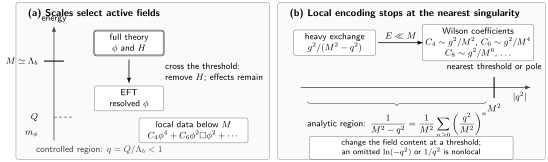
On a narrow screen, swipe the diagram or focus it and use the left/right arrow keys; Home and End move to its edges. Open the full-size diagram.
Scale separation selects the resolved states. Below the illustrative heavy scale , remains active and heavy virtual effects enter local coefficients. The dimensionless counting parameter is ; the exchanged four-momentum has mass dimension one. The heavy propagator’s geometric series converges for , while light nonanalytic propagation must remain dynamical. The diagram shows the tree-level hard contribution and is schematic, not to scale.
Exact heavy exchange and its local expansion
Section titled “Exact heavy exchange and its local expansion”In four spacetime dimensions, consider a real scalar with zero tree-level mass and a real scalar of tree-level mass ,
Take real , , and weak dimensionless couplings and . The potential completes to
Thus the origin is the stable classical vacuum. Without the stabilizing quartic the potential would be unbounded and the massless origin would not be a local minimum. Here the light contact interaction is retained unchanged in both theories. This is a tree-level benchmark; radiative mass tuning, loop matching, and quantum vacuum stability require additional analysis.
For , let denote the heavy-exchange contribution, with the overall Feynman-rule factor removed. Keeping the heavy denominators unexpanded gives
The complete tree amplitude in the site’s convention is
The three exchange signs follow from two vertices and one propagator in each channel; the contact rule is , as on Scalar Contact and Exchange Amplitudes. All formulas below stay below the heavy poles, where the tree boundary value is real.
Below all heavy poles, each channel has the geometric expansion
Keeping the local series through gives
For massless on-shell scattering, , so the nominal contribution cancels in this observable. To see what that means for the action, complete the Gaussian square in . Its equation is , giving the induced interaction
This is an unreduced operator expansion. With vanishing boundary terms, integration by parts gives
A perturbative local field redefinition can therefore use the leading light-field equation of motion to trade this derivative term for other interactions. The leading matched quartic is , so produces a six-field interaction. The induced higher-order terms must be retained to the requested accuracy, and sources must be transformed when comparing off-shell correlation functions. The four-point kinematic zero alone does not justify simply discarding these effects. This distinction between an unreduced expansion and a reduced basis follows the order-by-order construction in Burgess 2021, § 2.5, pp. 45–46. The full elimination is developed in Integrating Out Heavy Fields.
At fixed center-of-mass angle , use
Then
The first omitted contribution is therefore
Normalizing the truncation error by the exact exchange contribution gives
The residual therefore approaches slope six on a log–log plot against . An exact remainder also turns the expansion into a finite accuracy statement. Define
Subtracting the retained polynomial from each heavy denominator gives
Here every invariant is real and . For the fixed angle above, and . Moreover, is convex for . Since , averaging the three values yields . Hence
The bound increases with on . Thus choosing guarantees : retaining the quadratic invariant terms meets, for example, a target exchange-relative accuracy of throughout this window. This conservative bound controls the tree-level truncation, not omitted loop contributions.
For the total amplitude, keep the same contact term:
The absolute amplitude error is unchanged by the common contact term. Its relative error can be amplified near a cancellation in the total amplitude and is undefined at an exact zero. A cross-section uncertainty must instead compare the complete squared amplitudes with the same phase space. The stable completion therefore preserves the exchange benchmark without turning its relative error into a universal observable error.
Numerical residual check
Section titled “Numerical residual check”For the chapter fixture , in consistent mass units, the exact exchange contribution and its expansion through give the following values. These columns apply for any common ; the total amplitude is obtained by subtracting that same from both amplitude columns.
| Exact exchange | EFT exchange | Exchange-relative residual | |
|---|---|---|---|
| 0.050 | 0.03000009733 | 0.03000009722 | |
| 0.075 | 0.03000049339 | 0.03000049219 | |
| 0.100 | 0.03000156234 | 0.03000155556 | |
| 0.150 | 0.03000795409 | 0.03000787500 | |
| 0.200 | 0.03002534746 | 0.03002488889 | |
| 0.250 | 0.03006258503 | 0.03006076389 | |
| 0.300 | 0.03013171112 | 0.03012600000 |
An unweighted linear fit to versus over these seven points gives slope . The small excess above six is expected because the exact residual contains higher powers. Restricting the fit toward smaller approaches the analytic slope six; omitting the term instead gives a leading slope of four.
A slope checks the leading power, but cannot establish the normalization. At fixed , replacing by the numerical value of in fixed units only translates the horizontal logarithmic coordinate, leaving the slope unchanged. A constant multiplicative error in likewise translates the vertical coordinate. The dimensionless axis, stated parameters and direct amplitude/residual comparisons in the table are therefore separate checks.
A reproducible calculation is designed around this deterministic benchmark and adds explicit adversarial cases. The table above preserves the reference claim independently of an interactive implementation.
Top-down and bottom-up EFTs
Section titled “Top-down and bottom-up EFTs”When the full theory is known, one can integrate out or match its heavy degrees of freedom. The coefficients are then calculable functions of the heavy masses, couplings, renormalization scheme, and matching scale. The exact tree-level heavy-exchange calculation, combined with the retained contact interaction, is such a top-down construction. In particular, the leading matched quartic is .
When the ultraviolet completion is unknown, locality and symmetry still determine the operator structures. Their coefficients are independent low-energy parameters to be measured or constrained. This bottom-up construction remains predictive because only finitely many combinations contribute at a declared order. Measurements can then reveal which symmetries are approximate, estimate , and test whether the assumed counting is self-consistent.
The two viewpoints share the same low-energy action. They differ in how its coefficients are obtained and what correlations among them are justified. A bottom-up coefficient should not be assigned a heavy-mediator relation merely because that relation holds in one possible completion. Conversely, matching a known full theory without including every EFT operator required at the retained order makes the comparison incomplete.
Burgess constructs the low-energy generator and Wilson action, then organizes their local interactions by dimensions and scaling Burgess 2021, §§ 2.2–2.4, pp. 26–44.
What systematic improvement does and does not promise
Section titled “What systematic improvement does and does not promise”Systematic improvement means that a larger calculation comes with a sharper residual prediction. It does not mean that every series converges indefinitely. Perturbative coefficients may eventually grow, several small parameters may compete, or a new threshold may reorganize the degrees of freedom. The useful claim is local in theory space and kinematics: within a tested window, the retained hierarchy orders contributions and the residual behaves accordingly.
The statement also does not guarantee naturally sized coefficients. A symmetry can suppress a coefficient; a resonance can enhance one; an infrared fine tuning can promote an interaction; and a poor normalization can make dimensionless coefficients appear large. Coefficient sizes become evidence only relative to a specified normalization and mechanism.
Finally, an EFT does not erase ultraviolet physics. Heavy effects survive in Wilson coefficients, threshold corrections, anomalies, and the values of relevant parameters. What decouples is the need to resolve the detailed heavy dynamics in every low-energy calculation. The assumptions behind that statement are examined in Decoupling Theorems and Threshold Corrections.
Common pitfalls
Section titled “Common pitfalls”“Nonrenormalizable” means unpredictive. An interaction with canonical dimension greater than four requires additional counterterms, but an EFT includes them in a hierarchy. Predictivity is an order-by-order claim, tested by Loops, Counterterms, and Closure of an EFT Expansion.
The regulator cutoff is the breakdown scale. A regulator is an intermediate definition; is a property of the chosen physical description. Cutoff variation can diagnose missing counterterms, but setting the regulator equal to a heavy mass does not prove the EFT is valid up to that mass.
A small correction proves the expansion. A single accidental cancellation can make one order tiny. Control requires the predicted scaling across energies or observables and stability under the complete contribution set.
Integrating out means deleting a field. Eliminating produces a generally nonlocal functional of ; the local EFT is its low-energy expansion. In this model the Gaussian kernel is independent of , so its determinant contributes only to vacuum normalization. A background-dependent heavy kernel can instead generate field-dependent loop interactions, as explained in Integrating Out Heavy Fields.
Exercises
Section titled “Exercises”For the fixed-angle heavy-exchange fixture, truncate the amplitude after the term. What residual slope is expected even though ?
Solution
On shell the entire contribution cancels, so this truncation equals the leading result . The first nonzero correction is
Relative to , the residual begins as . The expected log–log slope is four, not two. The absent quadratic correction is an observable-specific kinematic cancellation.
Suppose a full amplitude contains from a massless light-particle cut, where is a reference mass scale. The retained kinematic domain resolves the nonanalytic dependence on near the light threshold. Can its entire effect be absorbed into a momentum-independent Wilson coefficient after the light particle is removed?
Solution
No. The logarithm is nonanalytic at the light threshold and represents propagation over resolved distances. A momentum-independent coefficient is analytic in the low external invariants. The light degree of freedom, or an equivalent nonlocal structure, must remain in the effective description; only the hard analytic part can be assigned to local Wilson coefficients.
References
Section titled “References”- Burgess, C. P. Introduction to Effective Field Theory: Thinking Effectively about Hierarchies of Scale. Cambridge: Cambridge University Press, 2021. DOI
Further reading
Section titled “Further reading”- Weinberg, Steven. “Phenomenological Lagrangians.” Physica A: Statistical Mechanics and its Applications 96, nos. 1–2 (1979): 327–340. DOI