Regulators, Cutoffs, and Continuum Limits

A regulator is the complete modification or construction that makes specified quantum-field-theory objects well defined; a cutoff is one scale or parameter within those data and may be auxiliary or physically retained. An interacting continuum theory is claimed only for a tuned family with matched observables, held-fixed renormalized data, ordered limits, a stated mode of convergence, checks of the structural properties being claimed, and controlled errors. Comparing independently regulated families is additionally required when cross-regulator universality is claimed. Finite results at several cutoffs—or regulator cancellation order by order—are evidence at their stated level, not automatically a nonperturbative existence theorem.

Required background. What an Interacting Lagrangian Does and Does Not Specify identifies the missing state, observable, regulator, renormalization, and limit data. Regulated Bosonic Field Integrals supplies the finite measure and keeps regulator removal distinct from the volume limit.

Helpful background. Limits, Completeness, and Convergence supplies the topology and convergence language; Lebesgue Integration and Convergence Theorems states when a limit may be interchanged with an integral.

A regulated family and its target observables

Regulation is more than attaching a symbol $\Lambda$ to an integral. A regulated member of a family must specify enough data to construct the quantities being compared. Schematically, write

$$\mathfrak T_{\mathcal R} =\left( \mathcal X_{\mathcal R}, S_{\mathcal R}\ \text{or}\ H_{\mathcal R}, \omega_{\mathcal R}, \mathbf g_0(\mathcal R), \{O_{i,\mathcal R}\} \right).$$

Here $\mathcal R$ can include a lattice or momentum cutoff, volume and boundary conditions, mode truncation, operator domains, measure, or switching data. The bare coordinates $\mathbf g_0(\mathcal R)$ generally vary with the regulator. The state $\omega_{\mathcal R}$ and regulated observables $O_{i,\mathcal R}$ are part of the construction, not optional decorations.

Four nearby terms should remain distinct:

• A regulator is the full prescription that makes the chosen objects meaningful.
• A cutoff is a scale or finite parameter within that prescription, such as $a$, $\Lambda$, a volume, or a maximum mode number.
• A renormalization prescription defines physical input parameters and composite observables through stated conditions, usually at a scale $\mu$.
• A physical ultraviolet scale may be deliberately retained in an effective theory; not every well-posed question asks for its removal.

A continuum claim starts with a target observable class and a tuning rule

$$\mathbf g_0(\mathcal R) =\mathbf g_0\!\left(\mathcal R;\mathbf g_R,\mu\right),$$

where the renormalized data $\mathbf g_R$ are held fixed while the auxiliary regulator is changed. The central question is then whether matched quantities $Q_{\mathcal R}[O_{\mathcal R}]$ approach a regulator-independent limit in a declared sense. Zinn-Justin’s cutoff and lattice discussions make this dependence on tuning, critical scaling, and renormalized data explicit Zinn-Justin 2021, § 8.4, printed pp. 166–169; § 8.7, printed pp. 175–176; and § 9.2, printed pp. 187–191.

The cutoff scalar as a complete claim

Return to the real scalar, now on a periodic $d$-dimensional lattice with spacing $a$, $N$ sites in each direction, and physical extent $L=Na$. Define a dimensionless lattice field and bare coordinates by

$$\varphi_n=a^{(d-2)/2}\phi(x_n), \qquad \widehat m_0^2(a)=a^2m_0^2(a), \qquad \widehat\lambda_0(a)=a^{4-d}\lambda_0(a).$$

One regulated action is

$$S_{a,N}[\varphi] =\sum_{n\in\mathbb Z_N^d} \left[ \frac12\sum_{\mu=1}^{d} (\varphi_{n+\hat\mu}-\varphi_n)^2 +\frac12\widehat m_0^2(a)\varphi_n^2 +\frac{\widehat\lambda_0(a)}{4!}\varphi_n^4 \right], \qquad \widehat\lambda_0(a)>0.$$

Because $\widehat\lambda_0(a)>0$, the finite-dimensional weight is integrable:

$$Z_{a,N} =\int_{\mathbb R^{N^d}} e^{-S_{a,N}[\varphi]} \prod_{n\in\mathbb Z_N^d}\mathrm d\varphi_n <\infty, \qquad \mathrm d\mu_{a,N}(\varphi) =\frac{e^{-S_{a,N}[\varphi]}}{Z_{a,N}} \prod_{n\in\mathbb Z_N^d}\mathrm d\varphi_n.$$

Thus the action together with the integration domain, periodic boundary conditions, and normalization defines a finite-dimensional Euclidean probability model. To state a massive continuum target, choose renormalized conditions—for example, a physical correlation length $\xi=m_R^{-1}$ and a dimensionless four-point coupling $g_R$—and tune $\widehat m_0^2(a)$ and $\widehat\lambda_0(a)$ so that those quantities remain fixed.

The correlation length measured in lattice units is

$$\widehat\xi(a)=\frac{\xi}{a}.$$

A continuum scaling limit requires

$$\frac{\xi}{a}\longrightarrow\infty,$$

while an infinite-volume limit independently requires

$$\frac{L}{\xi}=\frac{N}{\widehat\xi}\longrightarrow\infty.$$

Thus $a\to0$ and $L\to\infty$ answer different questions. Sending $a$ to zero while freezing arbitrary dimensionless bare lattice coordinates is generally not the desired trajectory: away from a critical surface, $\widehat\xi$ can remain finite and no nonzero physical correlation length survives. The critical-scaling interpretation of a lattice continuum limit is developed in Zinn-Justin 2021, § 8.7, printed pp. 175–176.

For a matched regulated observable, the desired claim has the form

$$\begin{aligned} Q[O] &=\lim_{k\to\infty}Q_{a_k,N_k}[O_{a_k,N_k}] \Big|_{m_R,\,g_R,\,\mu\ \mathrm{fixed}},\\ \frac{\xi}{a_k}&\longrightarrow\infty, \qquad \frac{N_k a_k}{\xi}\longrightarrow\infty. \end{aligned}$$

The sequence declares a joint scaling path; an iterated limit is a particular alternative and must name its order. This formula is a contract to be justified, not a proof. It must be accompanied by the observable definition, tuning procedure, convergence mode, finite-volume control, restored properties, and error statement.

What must converge

Bare fields and composite monomials need not have regulator-independent normalization. A matched continuum operator can involve rescaling and mixing,

$$O_{i,\mathcal R}^{R}(\mu) =\sum_j Z_{ij}(\mathcal R,\mu)\,O_{j,\mathcal R}.$$

The continuum statement should therefore concern a declared class of renormalized quantities: smeared correlation distributions, dimensionless ratios, spectral gaps, matrix elements, response coefficients, or another physical observable. It should say whether convergence is pointwise, distributional, weak, strong, in norm, in probability, or only an extrapolation within a fitted scaling ansatz.

The following data belong next to every displayed limit:

1. the regulator family and its admissible parameter domain;
2. the tuned bare trajectory and held-fixed renormalized conditions;
3. the matched observable or operator-mixing prescription;
4. the order of infinite-volume, continuum, source, and other limits;
5. the topology or mode of convergence;
6. the structural properties claimed for the limit; and
7. the error bound, uncertainty model, or theorem hypotheses.

Comparing bare couplings or field normalizations across schemes is usually not a universality test. Dimensionless physical ratios and consistently normalized renormalized observables are better comparison coordinates.

From regulator data to a continuum claim

The figure summarizes the logical chain, using $\rho$ for a generic regulator coordinate and $\rho_\star$ for its removal endpoint. Inspect the side labels as carefully as the main arrows: perturbative cancellation, numerical scaling, and a constructive proof support different strengths of conclusion.

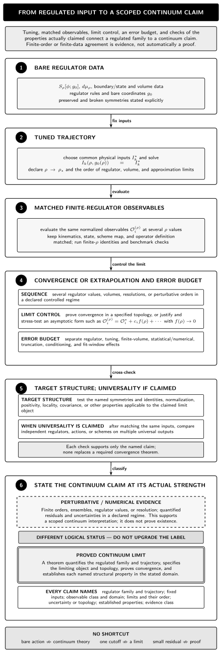
A regulated family supports a continuum claim only after the bare data are tuned along a trajectory fixed by common inputs, the same observables are matched at several regulator values, the removal limit is controlled by a justified convergence or extrapolation analysis with a full error budget, and the target structural properties are checked. Cross-regulator comparison is additionally required when universality across independently regulated families is claimed. Finite-order perturbative or finite-data numerical agreement is evidence in a declared regime, not a proof. A proved continuum limit additionally specifies the limiting object and topology and establishes convergence and the claimed properties by theorem. The map is schematic and not to scale.

The table supplies the complete nonvisual version of the map.

Stages and evidence in an interacting continuum claim

Stage	Required information	What it can establish	What it does not establish
Bare regulator data	Regulated object, cutoff parameters, volume, boundaries, state, and bare coordinates	A well-defined finite-regulator calculation or formal construction	A physical renormalization condition or continuum target
Tuned trajectory	Held-fixed renormalized quantities and a rule for changing bare data with the regulator	A family aimed at one declared physical target	Convergence, uniqueness, or regulator independence
Matched observables	Operator normalization or mixing, state matching, and common physical units	Meaningful comparison among members of the family	That a finite list determines the complete continuum theory
Convergence or extrapolation	Limit order, topology or scaling ansatz, fit range, and finite-volume and cutoff control	A limit theorem, perturbative cancellation, or numerical estimate at its stated level	A stronger existence statement than the method and hypotheses support
Error budget	Statistical, discretization, finite-volume, tuning, truncation, matching, fit, and algorithmic effects with correlations	A quantified range of reliability	Zero uncertainty because several regulators agree
Universality and structural checks	Tests of symmetries, positivity, locality, spectra, or target axioms; cross-regulator matching when universality is claimed	Evidence or proof that the limit has the declared physical identity, plus cross-family robustness when tested	Automatic equivalence of every observable, state, or sector
Scoped continuum claim	The exact observable class, regime, construction, convergence status, and residual limitations	Only the conclusion supported by the preceding chain	A universal claim extending beyond its object class and hypotheses

Evidence is graded, not binary

Several kinds of success are valuable, but they answer different questions.

Exact finite-regulator identity. An identity in a finite lattice model or cutoff Hamiltonian is exact for that regulated object. Its cutoff dependence remains part of the result.

Perturbative regulator cancellation. Counterterms can remove auxiliary-regulator dependence through a specified order for a specified observable. One must still give the renormalized inputs, scale and scheme, truncation uncertainty, and infrared qualifications. Order-by-order cancellation is not by itself a nonperturbative existence proof.

Numerical scaling and extrapolation. A continuum estimate needs a scaling regime and must control statistical, finite-volume, discretization, tuning, fit-model, autocorrelation, and algorithmic effects. These terms can be correlated; they should not be added in quadrature without a covariance or independence justification.

Cross-regulator universality. Agreement after matching the same renormalized data is stronger than stability inside one discretization. It remains conditional on the observable class, scaling window, and precision tested.

Constructive theorem. A proof names the object, limiting topology, hypotheses, and structural properties. It need not provide the same numerical observables or approximation guarantees as a simulation. Constructive reviews show why cutoff removal and axiom verification are model-specific achievements Summers 2016, §§ 1 and 3, printed pp. 1–4 and 9–18 (PDF).

Universality is a conditional statement

Universality means that appropriately matched regulator families yield the same declared long-distance or continuum observables despite differences in microscopic coordinates. A fixed-point description explains how irrelevant directions can lose influence while relevant parameters must be tuned. The domain of attraction, dimensional setting, symmetry class, operator content, and observable matching are hypotheses, not consequences of using the same word “$\phi^4$” Wilson and Kogut 1974, §§ 1.1 and 12.3, printed pp. 78–83 and 168–172, Zinn-Justin 2021, § 17.3, printed pp. 426–428.

A regulator may also break a target symmetry. A hypercubic lattice does not possess exact continuum rotations or boosts; other regulators can obscure gauge or chiral symmetries. Restoration must be checked through Ward identities, dispersion relations, degeneracies, operator relations, or the relevant theorem. Positivity, locality, and unitarity likewise require construction-specific checks.

Common failure modes

“Finite at several cutoffs” is not “cutoff independent.” A preasymptotic plateau can occur outside the scaling regime. Vary the regulator on a matched trajectory and include the full error model.

Setting $a=0$ is not a procedure. The lattice theory exists for $a>0$. The continuum claim concerns a sequence of matched observables along tuned bare data as $\xi/a$ diverges.

Same symmetry is not automatic universality. Symmetry constrains the target class, but fixed-point attraction, relevant data, phases, and operator matching must also agree.

A restored two-point dispersion is not the whole theory. It tests one sector. Composite operators, higher correlators, states, and other structural properties can retain cutoff artifacts.

Regulator removal is not always the goal. In an effective theory, a finite physical cutoff and a controlled expansion may be the correct description. The error claim replaces an inappropriate demand for ultraviolet completion.

This page does not settle a model’s ultraviolet fate. Whether a particular four-dimensional scalar family has a nontrivial, Gaussian, or nonexistent continuum limit is a separate model-specific question. No conclusion follows from the formal quartic density alone.

Check your understanding

1. Distinguish a regulator from a cutoff.

Answer

The regulator is the full prescription defining the intermediate object: variables, action or Hamiltonian, measure or domains, volume, boundaries, and operator definitions. A cutoff is one finite scale or parameter inside that prescription.

2. Why is $a\to0$ at fixed $\widehat m_0^2$ and $\widehat\lambda_0$ generally the wrong lattice trajectory?

Answer

Generic fixed bare coordinates have a finite correlation length in lattice units. Then the physical correlation length $a\widehat\xi$ collapses as $a\to0$. A continuum target instead tunes toward a critical surface so $\widehat\xi=\xi/a\to\infty$ while selected renormalized quantities stay fixed.

3. What is missing from a smooth continuum-extrapolation plot?

Answer

One still needs the matched observable and tuning conditions, justified scaling ansatz and fit range, limit order, statistical correlations, finite-volume and discretization control, tuning and algorithmic errors, and a statement of which structural or universality claims were actually tested.

4. Where should the developed calculation go?

Answer

Use Renormalization and EFT for counterterms, running, matching, and perturbative regulator removal; Lattice and Hamiltonian QFT for discretization, lines of constant physics, and continuum extrapolation; and Mathematical QFT for constructive limits and axiom verification.

Where to continue

• Regulator Removal and Renormalized Predictions develops counterterms, scheme consistency, running, and finite predictions.
• Lattice Regulators and Target Continuum Theories develops discretization, tuning, scaling, and symmetry restoration.
• Continuum Limits and Universality Problems states rigorous existence and comparison questions.
• Gaussian Euclidean Fields and Measures and Euclidean Measures to Relativistic Models develop constructive measure and reconstruction steps.
• Haag’s Theorem: Physical Meaning and Scope is the next chapter page; it asks why a global free-field interaction picture is obstructed even after regulator questions are separated.

References

• Summers, Stephen J. “A Perspective on Constructive Quantum Field Theory.” arXiv:1203.3991v2 [math-ph], revised 2016 (originally submitted 2012). Stable record. Open PDF, v2.
• Wilson, Kenneth G., and John Kogut. “The Renormalization Group and the $\epsilon$ Expansion.” Physics Reports 12, no. 2 (1974): 75–199. DOI.
• Zinn-Justin, Jean. Quantum Field Theory and Critical Phenomena. 5th ed. Oxford University Press, 2021. DOI.