Wess–Zumino Consistency and Descent

The Wess–Zumino condition is the statement that an anomalous variation must still realize the algebra of the symmetry transformations. For a consistent anomaly—one obtained from a single effective action—this condition is forced by the commutator of two variations. In BRST language it becomes a ghost-number-one cocycle condition. Descent then turns a closed invariant characteristic form in two higher degrees into a local consistent anomaly representative in the physical dimension.

This page develops that local perturbative chain with all form degrees, ghost numbers, and signs explicit. The characteristic polynomial is a universal or formal degree-$(d+2)$ object, not an ordinary nonzero $(d+2)$-form on the physical $d$-manifold. Chern–Simons and descent forms are local representatives; boundaries, nontrivial bundles, large transformations, and torsion require additional data.

Required background. What Is an Anomaly? supplies the counterterm quotient and the distinction between gauge and background anomalies. Differential Forms, Integration, Orientation, and Stokes Theorem supplies graded products, pullbacks, and Stokes’ theorem. de Rham Cohomology, Periods, Duality, and Intersection supplies closed-versus-exact reasoning and the global warning behind local primitives.

Helpful background. BRST Cohomology and Physical Observables supplies kernel-modulo-image reasoning and relative local cohomology. Characteristic Classes and Chern–Weil Theory supplies invariant polynomials and characteristic-form normalization.

Closure of gauge variations is the consistency condition

Let $W_E[\mathcal A]$ be a Euclidean effective action for a Hermitian matrix-valued background connection. Absorb couplings and charges into $\mathcal A$ and define

$$\mathcal F=\mathrm d\mathcal A-i\mathcal A^2, \qquad \delta_\Lambda\mathcal A=D\Lambda =\mathrm d\Lambda-i[\mathcal A,\Lambda].$$

All products of forms below are wedge products. In this convention the commutator of two infinitesimal transformations closes as

$$[\delta_{\Lambda_1},\delta_{\Lambda_2}] =\delta_{\Lambda_{12}}, \qquad \Lambda_{12}=-i[\Lambda_1,\Lambda_2].$$

Define the integrated consistent anomaly functional by

$$\mathfrak A_{\mathrm{cons}}(\Lambda) :=\delta_\Lambda W_E.$$

Applying the commutator to the same functional $W_E$ gives

$$\begin{aligned} &\delta_{\Lambda_1}\mathfrak A_{\mathrm{cons}}(\Lambda_2) -\delta_{\Lambda_2}\mathfrak A_{\mathrm{cons}}(\Lambda_1) \\ &\hspace{7em} =\mathfrak A_{\mathrm{cons}} \bigl(-i[\Lambda_1,\Lambda_2]\bigr). \end{aligned}$$

This is the Wess–Zumino consistency condition. It is an integrability condition: the anomalous Ward identity may fail, but its failure cannot violate the algebra obeyed by the transformations themselves. The original condition appears in Wess and Zumino 1971, pp. 95–97; a direct effective-action derivation with the gauge-algebra signs displayed is given in Bilal 2008, § 9.1, arXiv v1, pp. 70–71, eqs. (9.2)–(9.9), Open PDF.

The equation is necessary, not sufficient. A local expression can satisfy it even when its coefficient vanishes in the actual matter spectrum, and a solution can be removable by an admissible local counterterm. Conversely, the covariant current from the previous page is generally not a functional derivative of one $W_E$ and need not obey the non-Abelian Wess–Zumino condition. For an Abelian group the right-hand side vanishes, but the two variations must still commute. For the gauge-invariant $F\wedge F$-type densities used below, each variation vanishes separately and the condition is automatic.

BRST turns the algebra into a local cocycle equation

Replace the even parameter $\Lambda$ by an odd ghost $c$ and use a left BRST differential of ghost number one:

$$s\mathcal A=Dc, \qquad sc=i c^2, \qquad s^2=0.$$

On coefficient-valued forms, use the component convention inherited from the BRST prerequisite:

$$s\mathrm d=\mathrm d s.$$

Thus $s$ commutes with coordinate derivatives; no unspoken total-degree sign is being used. The ghost rule is precisely what encodes the commutator term in the Wess–Zumino equation. Replacing $\Lambda$ by $c$ turns that equation into

$$s\,\mathfrak A_{\mathrm{cons}}(c)=0.$$

To see the equivalence directly, introduce independent odd numbers $\eta_1,\eta_2$ and set

$$c=\eta_1\Lambda_1+\eta_2\Lambda_2, \qquad sc=-\eta_1\eta_2\Lambda_{12}.$$

The coefficient of $\eta_1\eta_2$ in $s\mathfrak A_{\mathrm{cons}}(c)$ is exactly the Wess–Zumino residual. At the density level that residual can be a total derivative:

$$\begin{aligned} &\delta_{\Lambda_1}Q_d^{(1)}(\Lambda_2) -\delta_{\Lambda_2}Q_d^{(1)}(\Lambda_1) -Q_d^{(1)}(\Lambda_{12}) \\ &\hspace{6em} =-\mathrm dQ_{d-1}^{(2)}(\Lambda_1,\Lambda_2). \end{aligned}$$

The integrated equality follows only when the surface term vanishes or is included in the problem.

An integrated local anomaly on a $d$-manifold has the form

$$\mathfrak A_{\mathrm{cons}}(c) =-2\pi i\int_X a_d^{\,1},$$

where the superscript is ghost number and the subscript is form degree. At the density level, closure is only required modulo a total derivative:

$$s a_d^{\,1}+\mathrm d a_{d-1}^{\,2}=0.$$

Two representatives define the same local class when

$$a_d^{\,1} \sim a_d^{\,1}+s b_d^{\,0}+\mathrm d b_{d-1}^{\,1}.$$

The $s b_d^{\,0}$ term is the variation of a local counterterm; the $\mathrm d b_{d-1}^{\,1}$ term integrates away only on a closed manifold or under stated support or boundary conditions. With those hypotheses, genuine local anomaly candidates lie in the relative cohomology

$$H^{1,d}(s\mid\mathrm d).$$

This statement is local: it uses a local algebra of fields, ghosts, and a finite number of derivatives. Its precise cohomological formulation and counterterm equivalence are developed in Barnich, Brandt, and Henneaux 2000, §§ 2.2–2.3, arXiv v3, pp. 7–11, especially eq. (2.23), Open PDF. The simpler BRST conversion of the Wess–Zumino condition appears in Bilal 2008, § 9.2, arXiv v1, pp. 71–73, eqs. (9.10)–(9.15), Open PDF.

Characteristic forms generate a descent staircase

Let $P_{d+2}$ be an invariant closed characteristic polynomial of total form degree $d+2$. On a local trivialization, the Poincaré lemma provides a Chern–Simons primitive $Q_{d+1}^{(0)}$. Successive BRST variations produce the descent equations. We choose the sign convention

$$\begin{aligned} P_{d+2}&=\mathrm d Q_{d+1}^{(0)}, \\ sQ_{d+1}^{(0)}&=\mathrm d Q_d^{(1)}, \\ sQ_d^{(1)}&=-\mathrm d Q_{d-1}^{(2)}, \\ &\hspace{1.2em}\vdots \end{aligned}$$

with $s\mathrm d=\mathrm d s$. The minus sign in the final displayed equation fixes the otherwise conventional sign of $Q_{d-1}^{(2)}$ and puts the result directly in the standard relative-cocycle form $s a+\mathrm d b=0$. The first descendant $Q_d^{(1)}$ is the consistent anomaly form; the next equation is its local Wess–Zumino consistency relation.

For an invariant polynomial

$$P_{2n+2}=\kappa\,\operatorname{tr}(\mathcal F^{n+1}),$$

a useful local transgression in the present Hermitian convention is

$$\begin{aligned} Q_{2n+1}^{(0)} &=(n+1)\kappa\int_0^1\mathrm dt\, \operatorname{tr}(\mathcal A\mathcal F_t^n), \\ \mathcal F_t &=t\,\mathrm d\mathcal A-i t^2\mathcal A^2. \end{aligned}$$

Direct differentiation gives $\mathrm dQ_{2n+1}^{(0)}=P_{2n+2}$. This construction and the first descendant are derived in Bilal 2008, §§ 8.3.2–8.3.3, arXiv v1, pp. 66–69, eqs. (8.50)–(8.74), Open PDF. The local-contractibility assumption behind a full descent tower is made explicit in Barnich, Brandt, and Henneaux 2000, §§ 9.1–9.2, arXiv v3, pp. 70–72, eqs. (9.1)–(9.4), Open PDF. A primary geometric account, including the local-versus-global qualification, is Zumino 1983/1984, §§ 2–4, LBL-16747, printed pp. 7–29, Open PDF; the higher-dimensional construction is also developed in Zumino, Wu, and Zee 1984, pp. 477–507.

The diagram organizes the $d=4$ case by bidegree. Read downward: each BRST variation is, up to the displayed sign, an exterior derivative of the next descendant. Read the dashed side branch only as the orientation for the next page: a five-dimensional bulk term can cancel the four-dimensional boundary variation only after its global definition, extension, and boundary data have been supplied.

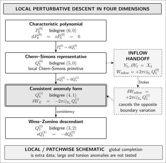
Local $d=4$ descent by form degree and ghost number. Solid relations are the local equations $P_6=\mathrm dQ_5^{(0)}$, $sQ_5^{(0)}=\mathrm dQ_4^{(1)}$, and $sQ_4^{(1)}=-\mathrm dQ_3^{(2)}$. The dashed inflow branch is schematic: it requires a globally defined bulk or differential-cohomological completion and does not test large or torsion anomalies.

Swipe horizontally to inspect the full diagram, or open the vector figure at full size.

The same relationships remain available without the image:

Objects in the local four-dimensional descent staircase

Object	Bidegree (form, ghost)	Role	Defining local relation
P₆	(6, 0)	Invariant universal characteristic polynomial	dP₆ = sP₆ = 0
Q₅⁽⁰⁾	(5, 0)	Local Chern–Simons representative	P₆ = dQ₅⁽⁰⁾
Q₄⁽¹⁾	(4, 1)	Consistent anomaly form	sQ₅⁽⁰⁾ = dQ₄⁽¹⁾
Q₃⁽²⁾	(3, 2)	Wess–Zumino consistency descendant	sQ₄⁽¹⁾ = −dQ₃⁽²⁾

The dashed branch has the following exact text equivalent. If a globally admissible completion exists on $Y_5$ with induced boundary $\partial Y_5=X_4$, the local inflow orientation is

$$\begin{aligned} W_{E,\mathrm{inflow}} &=+2\pi i\int_{Y_5}Q_5^{(0)}, \\ \delta W_{E,\mathrm{inflow}} &=+2\pi i\int_{X_4}Q_4^{(1)}. \end{aligned}$$

The second line cancels a boundary variation $-2\pi i\int_{X_4}Q_4^{(1)}$. This is only the local infinitesimal sign check; it does not establish that the exponentiated bulk term is globally defined or extension-independent.

The figure is a local schematic, not a claim that the Chern–Simons form is globally defined. On overlaps of trivializations its representatives differ by further descent data. Differential-cohomological refinement belongs to the mathematical continuation named below.

A four-dimensional Weyl fermion fixes the normalization

Now take a closed oriented Euclidean spin four-manifold $X$ and one physical Lorentzian left-handed Weyl fermion. Under the site’s Wick continuation it has negative Euclidean chirality. For a representation $R$, the universal six-form is

$$I_6^L =-\frac{1}{6(2\pi)^3}\operatorname{tr}_R(\mathcal F^3) +\frac{p_1(TX)}{24(2\pi)}\operatorname{tr}_R\mathcal F.$$

Here $I_6^L$ is a formal characteristic polynomial, equivalently a degree-six class evaluated after pullback to suitable auxiliary or family data. It is not an ordinary nonzero six-form on $X$. The mixed term is written in the representative that preserves diffeomorphism and local-Lorentz covariance and places the mixed violation in the gauge Ward identity.

A local Chern–Simons representative is

$$\begin{aligned} Q_5^{(0),L} &=-\frac{1}{16\pi^3}\int_0^1\mathrm dt\, \operatorname{tr}_R(\mathcal A\mathcal F_t^2) \\ &\quad+\frac{p_1(TX)}{48\pi} \operatorname{tr}_R\mathcal A. \end{aligned}$$

Its first descendant can be chosen as

$$\begin{aligned} Q_4^{(1),L}(\Lambda) &=-\frac{1}{48\pi^3} \operatorname{tr}_R\!\left[ \Lambda\,\mathrm d\!\left( \mathcal A\,\mathrm d\mathcal A -\frac{i}{2}\mathcal A^3 \right) \right] \\ &\quad+\frac{p_1(TX)}{48\pi} \operatorname{tr}_R\Lambda. \end{aligned}$$

Thus

$$\delta_\Lambda W_E =-2\pi i\int_X Q_4^{(1),L}(\Lambda).$$

Multiplying $Q_4^{(1),L}$ by $2\pi$ reproduces exactly the consistent four-form convention on the preceding Consistent and Covariant Anomalies page. The degree-six index normalization and chirality reversal follow from Álvarez-Gaumé and Vázquez-Mozo 2024, §§ 2–3, arXiv v2, pp. 4–8 and 10, eqs. (4)–(11), (17)–(19), and (22), Open PDF. The four-dimensional consistent descendant is worked out in Bilal 2008, §§ 9.3–9.4, arXiv v1, pp. 73–78, eqs. (9.16)–(9.41), Open PDF, after translating from Bilal’s anti-Hermitian connection and opposite chirality naming.

Abelian gauge and gravitational backgrounds

For one compact $U(1)$ charge $q\in\mathbb Z$, write $\mathcal A=q a$ and let $f=\mathrm da$ locally. The curvature $f$ is global even when the potential $a$ is not. Set

$$c_1=\frac{f}{2\pi}, \qquad p_1(TX)=-\frac{1}{8\pi^2} \operatorname{tr}_{\mathrm{vec}}(\mathcal R^2).$$

On a trivializing patch, introduce an Abelian ghost $\omega$ with $sa=\mathrm d\omega$ and $s\omega=0$. Then

$$I_6^L =-\frac{q^3}{6}c_1^3 +\frac{q}{24}c_1p_1(TX),$$

and one especially transparent descent is

$$\begin{aligned} Q_5^{(0),L} &=\frac{a}{2\pi} \left[-\frac{q^3}{6}c_1^2 +\frac{q}{24}p_1(TX)\right], \\ Q_4^{(1),L} &=\frac{\omega}{2\pi} \left[-\frac{q^3}{6}c_1^2 +\frac{q}{24}p_1(TX)\right]. \end{aligned}$$

Because the bracketed four-form is closed,

$$\mathrm dQ_5^{(0),L}=I_6^L, \qquad sQ_5^{(0),L}=\mathrm dQ_4^{(1),L}, \qquad sQ_4^{(1),L}=0.$$

The effective-action variation is therefore

$$sW_E =-i\int_X\omega \left[-\frac{q^3}{6}c_1^2 +\frac{q}{24}p_1(TX)\right].$$

This calculation separates two jobs. The index polynomial fixes the coefficient, including the chirality sign. Descent fixes the consistent local representative and its Wess–Zumino completion. Descent alone cannot predict whether the sum over a particular fermion spectrum vanishes. Opposite chirality flips the entire expression. The term proportional to $c_1p_1$ is a mixed gauge–gravity anomaly; four-dimensional spin-$\tfrac12$ fields have no perturbative pure gravitational anomaly.

Representative shifts, boundaries, and global limits

The descent representative is not unique. At ghost number one and form degree $d$,

$$Q_d^{(1)} \longmapsto Q_d^{(1)}+sB_d^{(0)}+\mathrm dB_{d-1}^{(1)}.$$

The first term is generated by the local counterterm

$$W_E\longmapsto W_E-2\pi i\int_X B_d^{(0)}.$$

It changes the representative but not a nontrivial class. In particular, if $Q_d^{(1)}=sB_d^{(0)}+\mathrm dB_{d-1}^{(1)}$, the opposite counterterm $+2\pi i\int_XB_d^{(0)}$ cancels the anomaly on a closed $X$, provided the counterterm is globally defined and admissible. The second term does not change the integrated anomaly on a closed $X$, but on a manifold with boundary

$$\int_X\mathrm dB_{d-1}^{(1)} =\int_{\partial X}B_{d-1}^{(1)}.$$

Likewise, the next descent equation gives

$$s\int_X Q_d^{(1)} =-\int_{\partial X}Q_{d-1}^{(2)}.$$

Therefore the ordinary integrated Wess–Zumino condition requires a closed manifold, compact support or falloff, boundary conditions that kill the surface term, or an enlarged boundary/inflow system. A transformation that changes the prescribed boundary data is not automatically a gauge redundancy of the same problem; a boundary-nonzero transformation may carry a charge. The support assumption used in the standard local derivation is stated explicitly in Bilal 2008, opening of § 9, arXiv v1, p. 69, eq. (9.1), Open PDF. A Maxwell example in which only boundary-vanishing transformations are quotiented while nonzero boundary values generate charges is given in Harlow and Wu 2020, Introduction and § 3.3, arXiv v4, pp. 1–3 and 26–27, eqs. (3.18)–(3.25), Open PDF.

Three further limits matter:

• A Chern–Simons form such as $Q_5^{(0)}$ is generally only local on a nontrivial bundle. Its patching, periods, and exponentiation require global information.

• Relative local cohomology detects infinitesimal, perturbative anomaly data. It does not by itself detect large-gauge phases, determinant-line holonomy, torsion, or dependence on the global form of the symmetry group.

• The descent of an invariant polynomial supplies an important family of cocycles, but a full classification depends on the chosen local complex, spacetime dimension, gauge algebra, Abelian factors, antifields, and regularity hypotheses. It is not a universal replacement for computing $H^{1,d}(s\mid\mathrm d)$.

The first two limits motivate Anomaly Polynomials and Inflow and Global and Torsion Anomalies. The theorem-level classification of relative local classes belongs to Local BRST Cohomology, Consistent Deformations, and Currents, while Local Anomaly Descent and Wess–Zumino Consistency develops the mathematical descent and its hypotheses. Differential- cohomological and globally refined anomaly data are taken up in those mathematical and later physical continuations.

Computational companion. No runnable anomaly-descent calculation is currently available. The bidegrees, signs, and four-dimensional coefficient checks are therefore worked explicitly on this page.

What the condition does and does not prove

Implications in the local descent argument

Established input	Valid conclusion	Not implied
One effective action and a closing infinitesimal algebra	The consistent anomaly obeys Wess–Zumino consistency	The anomaly coefficient is nonzero or nonremovable
Nilpotency s² = 0 and the stated local domain	Ghost-number-one cocycles and coboundaries are defined	Quantum measure invariance or absence of global anomalies
Local Poincaré lemma and an invariant polynomial of degree d + 2	A local Chern–Simons form and descent tower can be constructed	A globally defined primitive on every bundle
a = s b + d n at ghost number one and top form degree	The local representative is removable under admissible closed/support assumptions	Its boundary term is physically irrelevant on a bounded region
Vanishing local polynomial and trace coefficients	The associated perturbative local anomaly vanishes	Freedom from large, torsion, or other global anomalies

Common pitfalls

Treating $I_6$ as an ordinary form on four-dimensional spacetime. It is a universal or auxiliary degree-six characteristic object whose descent produces a four-dimensional anomaly. Three two-forms wedged directly on a four-manifold vanish.

Calling every Wess–Zumino solution a genuine anomaly. Consistency is a cocycle condition. The coefficient may vanish, and an exact representative may be removed by an admissible local counterterm.

Dropping total derivatives in the presence of a boundary. A $\mathrm d$-exact shift changes a boundary term. Boundary conditions, allowed transformations, edge degrees of freedom, and inflow decide whether that term is removable.

Using the covariant anomaly in descent. Descent generates the consistent effective-action representative. The covariant current is a local Bardeen–Zumino improvement and generally fails the non-Abelian Wess–Zumino condition.

Reading local descent as a global classification. Large transformations, torsion phases, global group form, and determinant-line holonomy require separate tests.

Check your understanding

1. Starting from $sQ_5^{(0)}=\mathrm dQ_4^{(1)}$ and $s\mathrm d=\mathrm d s$, show that $sQ_4^{(1)}$ is locally exact and explain the chosen sign of $Q_3^{(2)}$.

Solution

Apply $s$ once more:

$$0=s^2Q_5^{(0)} =s\mathrm dQ_4^{(1)} =\mathrm d(sQ_4^{(1)}).$$

Thus $sQ_4^{(1)}$ is closed. On a contractible local patch, the Poincaré lemma gives $sQ_4^{(1)}=\mathrm dR_3^{(2)}$. Defining $Q_3^{(2)}=-R_3^{(2)}$ yields $sQ_4^{(1)}=-\mathrm dQ_3^{(2)}$. This local step is precisely where topology and boundary qualifications enter.

2. For the Abelian example, verify all three equations $\mathrm dQ_5^{(0)}=I_6$, $sQ_5^{(0)}=\mathrm dQ_4^{(1)}$, and $sQ_4^{(1)}=0$.

Solution

Let

$$K_4=-\frac{q^3}{6}c_1^2+\frac{q}{24}p_1(TX).$$

Because $\mathrm dK_4=0$, $\mathrm da=f=2\pi c_1$, $sa=\mathrm d\omega$, and $s\omega=0$,

$$\mathrm d\left(\frac{a}{2\pi}K_4\right)=c_1K_4=I_6,$$ $$s\left(\frac{a}{2\pi}K_4\right) =\frac{\mathrm d\omega}{2\pi}K_4 =\mathrm d\left(\frac{\omega}{2\pi}K_4\right),$$

and $s[(\omega/2\pi)K_4]=0$.

3. Show that a representative shift by $sB_4^{(0)}$ is produced by a local counterterm, and identify what fails on a manifold with boundary for the $\mathrm dB_3^{(1)}$ shift.

Solution

Adding $-2\pi i\int_XB_4^{(0)}$ to $W_E$ changes its BRST variation by $-2\pi i\int_XsB_4^{(0)}$. This is exactly the $sB_4^{(0)}$ change of the anomaly representative. By contrast,

$$\int_X\mathrm dB_3^{(1)} =\int_{\partial X}B_3^{(1)},$$

so the second shift is invisible only when the boundary term vanishes or is accounted for by allowed boundary data.

4. Explain why the Wess–Zumino condition does not distinguish the displayed consistent and covariant Abelian $F\wedge F$ representatives.

Solution

For $U(1)$, $[\Lambda_1,\Lambda_2]=0$, and the displayed curvature-only densities are themselves invariant under Abelian gauge transformations. Thus both sides of the consistency equation vanish. This does not make the condition empty for an arbitrary Abelian candidate; it means that these two particular representatives are not distinguished by it. Their distinction is instead functional integrability: the consistent current is a derivative of one effective action, whereas the covariant current generally has a nonzero functional curl.

5. A spectrum has vanishing local cubic and linear anomaly coefficients. What has and has not been established?

Solution

The perturbative local gauge and mixed gauge–gravity anomaly polynomial associated with those coefficients vanishes. Nothing in that calculation tests large transformations, torsion phases, the global form of the group, boundary consistency, or other nonperturbative anomaly data.

References

• Álvarez-Gaumé, Luis, and Miguel Á. Vázquez-Mozo. “Anomalies and the Green–Schwarz Mechanism.” In Handbook of Quantum Gravity, edited by Cosimo Bambi, Leonardo Modesto, and Ilya L. Shapiro, 2241–2284. Singapore: Springer, 2024. DOI. Open PDF, arXiv v2.

• Barnich, Glenn, Friedemann Brandt, and Marc Henneaux. “Local BRST Cohomology in Gauge Theories.” Physics Reports 338, no. 5 (2000): 439–569. DOI. Open PDF, arXiv v3.

• Bilal, Adel. “Lectures on Anomalies.” LPTENS-08/05, arXiv:0802.0634v1 [hep-th], 2008. Stable record. Open PDF, arXiv v1.

• Harlow, Daniel, and Jie-qiang Wu. “Covariant Phase Space with Boundaries.” Journal of High Energy Physics 2020, no. 10 (2020): 146. DOI. Open PDF, arXiv v4.

• Wess, Julius, and Bruno Zumino. “Consequences of Anomalous Ward Identities.” Physics Letters B 37, no. 1 (1971): 95–97. DOI.

• Zumino, Bruno. “Chiral Anomalies and Differential Geometry.” In Relativity, Groups and Topology II, edited by Bryce S. DeWitt and Raymond Stora, 1291–1322. Amsterdam: North-Holland, 1984. Open report LBL-16747/UCB-PTH-83/16.

• Zumino, Bruno, Yong-Shi Wu, and Anthony Zee. “Chiral Anomalies, Higher Dimensions, and Differential Geometry.” Nuclear Physics B 239, no. 2 (1984): 477–507. DOI.