

The Faddeev–Popov Construction
After a finite-mode or lattice regulator has turned the field integral into an ordinary finite-dimensional integral, a gauge condition can be used as a coordinate transverse to the gauge orbits. If the chosen condition meets each orbit once in a specified neighborhood, after stabilizers have been removed, the derivative of the gauge condition along the orbit is the Jacobian of this coordinate change. Its determinant converts the integral over redundant representatives into an integral over a local gauge slice.
This is the Faddeev–Popov construction. It is a local change-of-variables argument, not a theorem that one gauge condition gives a global quotient. This page derives the determinant and the gauge-fixed integral, including residual symmetry and boundary qualifications. The Grassmann representation of the determinant, gauge-parameter families, and loop implementation belong to later pages.
Required background. Gauge Orbits, Gauss Constraints, and Stabilizers supplies the distinction between an orbit direction and a stabilizer. Regulated Bosonic Field Integrals supplies the finite-regulator measure and change-of-variables language used below.
Helpful background. Constraints, Dirac Brackets, and Symplectic Reduction explains the corresponding reduction of a constrained phase space.
A circle orbit and one local representative
Section titled “A circle orbit and one local representative”The entire construction is visible in a two-dimensional integral. Let act on by
and let the action depend only on . Dividing the invariant integral by the orbit volume gives
Choose the gauge condition
At a point on its zero set, the derivative along the orbit is
The half-line , contains exactly one point from each nonzero orbit. Its gauge-fixed integral is therefore
This agrees with the quotient integral. The factor is not an additional interaction; it is the Jacobian from the angular orbit coordinate to the transverse coordinate .
The full line exposes two different failures that a formal derivation can hide. Every circle with meets that line at both and , which are exchanged by the residual rotation . Consequently,
Using on the full line counts the quotient twice. Using the signed determinant instead makes the two intersections cancel:
One must either select the half-line, divide by the residual , or otherwise specify how the two roots are treated. At the origin the whole group is a stabilizer and , so the orbit-to-slice coordinate change is singular.
The figure summarizes these relationships. Inspect the opposite signs at the two intersections, the residual half-turn, the stabilized origin, and the four counting prescriptions. Open the full-size SVG.
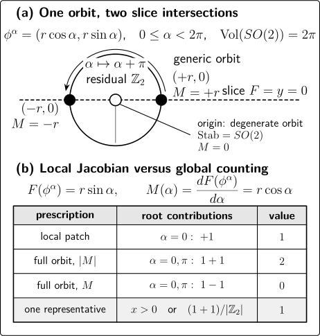
For on an orbit, the roots have . The modulus counts two intersections, whereas the signed determinant cancels them. Selecting or dividing by the residual restores one representative. The origin is stabilized by and has . The diagram is schematic and not to scale.
Text equivalent. Panel (a) shows the circle and the full horizontal slice . The roots at and have and ; the half-turn exchanges them and generates the residual . At the origin the orbit collapses, the whole group is a stabilizer, and . Panel (b) compares four counting prescriptions for the same orbit. A one-root local patch gives ; the full slice with gives ; the full slice with the signed gives ; and selecting or dividing by the residual gives . Thus the determinant is a valid transverse Jacobian on a local patch, but a global use must also control repeated intersections and stabilizers.
The local orbit-to-slice Jacobian
Section titled “The local orbit-to-slice Jacobian”Now let be a regulated configuration space, and let be the group of transformations that the theory declares to be redundancies. The subscript is consequential on a region with boundary: transformations carrying a physical surface charge are not included in merely because they preserve the boundary conditions.
For in the Lie algebra , write the infinitesimal action at as
A gauge condition with as many independent components as the orbit has local directions is a map
Its Faddeev–Popov operator is the derivative of along the orbit,
At a finite regulator, is an ordinary matrix. In continuum notation it is an operator whose domain includes the boundary or falloff conditions imposed on the allowed gauge parameters. In Euclidean one-loop boundary-value problems, the allowed gauge-parameter conditions become the ghost boundary conditions Vassilevich 2003, § 3.4, preprint pp. 27–29, Open PDF. A continuum functional determinant additionally requires a regularization and separate treatment of zero modes Vassilevich 2003, § 2.2, preprint pp. 14–16, Open PDF.
The local construction requires all of the following:
- the regulated action and measure are invariant under , or their transformation is included explicitly;
- on the chosen regular stratum, a declared effective group acts freely after any common kernel or stabilizer directions have been removed;
- the components of are independent in the directions being removed;
- within the chosen group neighborhood, has one root; and
- at that root is invertible.
The last two conditions are distinct. Invertibility makes one intersection transverse; it does not exclude another intersection elsewhere on the same orbit.
Fix a Haar volume form on the regulated group and a volume form on the target of . Determinants below are measured relative to those forms. Let . Using the invariant frame compatible with the chosen action convention, is represented by .
Suppose the roots in a group neighborhood are isolated and nondegenerate. The ordinary multidimensional delta-function identity then gives
In arbitrary coordinates, if , the same term is . Thus the group density is part of the determinant convention; it is not an extra constant that may be silently discarded.
On a one-root patch this becomes
where is the coordinate neighborhood containing the selected root . This is the real Faddeev–Popov identity. The modulus is required by the change-of-variables theorem Srednicki 2007, § 71, p. 421, eqs. (71.12)–(71.14).
The original perturbative prescription and its standard field-theory derivation write the unmodded determinant Faddeev and Popov 1967, pp. 29–30; Weinberg 1996, § 15.5, pp. 19–23. On a connected patch where never vanishes, its sign is constant, so an orientation can replace by the signed . That restricted determinant is the object represented by Grassmann ghosts on the next page. Across a zero of , or across several roots with different signs, the replacement is not valid without further information Vandersickel and Zwanziger 2012, §§ 2.1.2–2.1.4 and § 2.2.3, journal pp. 187–192 and 201.
From the identity to a gauge-fixed integral
Section titled “From the identity to a gauge-fixed integral”Let be a selected slice in a fixed regular stratum, and let be a gauge-saturated tube for which
is one-to-one. Also require : the selected slice is the entire zero set inside this tube, not merely one of several components. The effective group acts freely here, and the tube contains a complete orbit over each point of . For this local quotient chart, define the regulated Lorentzian integral
Insert the one-root identity in this tube, change variables along its complete orbits, and use invariance of and . The group coordinate now factors and cancels the same specified Haar volume, leaving
The absence of a prime records the free-action hypothesis, not an ignored zero mode. If a finite residual subgroup instead leaves representatives in the selected slice, the expression must be divided by , or the slice must be restricted to one representative. The half-line and its residual are the elementary version of this choice.
There is a different formula when a stabilizer is deliberately retained on a fixed orbit-type stratum. With compatible Haar normalizations, the transverse factor is : the prime removes the stabilizer directions, while the denominator removes their group volume. If stabilizer type or dimension jumps, no single smooth normalization covers both strata.
This argument constructs , not a global on all of . Reconstructing a global quotient requires compatible quotient charts and a partition of unity, or some other global prescription. The local identity alone cannot supply that prescription.
A useful normalization check is to replace the gauge condition by , where is a constant invertible matrix. Then
The two factors cancel. A formula that changes under this harmless reparametrization has lost either the delta-function Jacobian or the Faddeev–Popov determinant.
The based gauge group on a bounded region
Section titled “The based gauge group on a bounded region”Let be a smooth compact connected domain in Euclidean with boundary, and take a trivial principal -bundle. Take the field space to contain sufficiently regular connections whose pullback to is fixed. A transformation can preserve these field boundary conditions and still carry a nonzero charge. For Yang–Mills electric field , the generator of an infinitesimal transformation is
The bulk term is the Gauss constraint. The surface term can remain nonzero on the constraint surface and then generates a physical boundary symmetry. For the bounded application on this page, choose the based group
or infinitesimally . Its generators have no surface charge, and they preserve the fixed pullback of the connection. Boundary-preserving transformations with nonzero boundary value are not divided out; their classification continues in Proper and Improper Gauge Transformations.
This choice also fixes the domain of . Changing the allowed parameter space changes its kernel, determinant, and residual subgroup, so the boundary declaration cannot be appended after the calculation. For the continuum operators below, take
with regular enough for on this domain; the finite regulator uses the corresponding Dirichlet parameter subspace. Other field boundary data can change , the surface generator, and this operator domain.
Maxwell theory: field-independent does not mean structure-free
Section titled “Maxwell theory: field-independent does not mean structure-free”Use Coulomb gauge on ,
For Maxwell theory,
With the based group, obeys Dirichlet boundary conditions. The operator is independent of , and on a connected bounded region its Dirichlet kernel is trivial. Its determinant nevertheless depends on the geometry, regulator, and boundary conditions. At fixed geometry and boundary data it cancels from normalized gauge-field correlators; it need not cancel from an absolute partition function or from a comparison in which those data change.
On a compact boundaryless or periodic domain, a constant parameter lies in the kernel because it leaves the pure gauge field unchanged. It is a stabilizer direction and must be factored from the group volume and determinant. With charged matter or boundary data, whether a constant transformation is redundant is a physical declaration, not a conclusion drawn from the gauge-field formula alone.
Yang–Mills theory: the determinant depends on the field
Section titled “Yang–Mills theory: the determinant depends on the field”For compact Yang–Mills theory in the same gauge and conventions,
The plus sign follows from defining and . Sources that define either object with the opposite sign write instead; the determinant and ghost conventions must be translated together.
Because contains , the determinant is field dependent. At , or in the Abelian limit, it reduces to
which recovers the Maxwell result. This is an independent check on the normalization and index structure.
Two kinds of zero mode must not be conflated. A stabilizer satisfies
and therefore generates no displacement of . A nontrivial tangent zero mode satisfies
it generates an orbit direction tangent to the gauge slice, so the local inverse fails. In either case is not invertible. A zero eigenvalue does not, by itself, prove the existence of a second finite representative; that requires a global analysis.
The theorem-level construction of local slices uses functional-analytic hypotheses that the regulated derivation does not supply. Mitter and Viallet work on a principal bundle with compact, connected, semisimple matrix structure group over a compact finite-dimensional oriented Riemannian base without boundary. For Sobolev order , they obtain a free action either from the point-based subgroup on all connections or from the full gauge group modulo its center on irreducible connections; together with a tangent-space splitting, this yields local gauge sections Mitter and Viallet 1981, pp. 457–461 and 466–468. That result is not a theorem for the bounded region considered above. The exact boundary-capable or theorem-first hypotheses belong to Local Slices, Gauge Fixing, and Faddeev–Popov Geometry.
Checks and limits
Section titled “Checks and limits”One-root normalization. The half-slice reproduces the quotient integral exactly. The full slice gives two with the modulus and zero with the signed determinant. Both wrong answers diagnose an undeclared residual multiplicity or an invalid global orientation.
Gauge-condition reparametrization. The product is unchanged under . This checks the normalization without referring to a particular action.
Abelian limit. Sending the Yang–Mills commutator term to zero gives . A remaining field dependence would signal an inconsistent covariant-derivative convention.
Locality. A nonzero determinant at one configuration licenses a local transverse coordinate, not a global choice of one representative. Singer’s result proves the absence of a continuous global gauge choice for connections over with compact non-Abelian structure group Singer 1978, pp. 7–12, Open PDF. Its hypotheses must not be replaced by the claim that every gauge problem has the same obstruction.
Continuum status. The derivation is exact at the declared finite regulator. In continuum notation, the measure, determinant, integration cycle, and limit still require definitions. A formal determinant does not construct a nonperturbative quotient measure.
Common pitfalls
Section titled “Common pitfalls”Treating the group volume as a universal constant. Stabilizers and residual subgroups make the normalization configuration dependent or stratum dependent unless they are handled first. State the group, its measure, and every removed zero mode.
Using a local determinant as a global uniqueness test. The condition says that one crossing is transverse. It neither counts other crossings nor excludes them.
Calling every zero mode a Gribov copy. A zero mode may be a stabilizer or a nontrivial tangent direction. Even the latter establishes loss of local invertibility, not yet a second finite intersection.
Replacing the modulus without a sign declaration. The real delta-function identity contains . The signed determinant is appropriate only on a connected oriented patch where its sign is fixed.
Discarding every Abelian determinant. Maxwell’s determinant is independent of in a linear gauge, but it retains geometry, regulator, zero-mode, and boundary dependence. Specify the observable and normalization before cancelling it.
Dividing out charged boundary transformations. A transformation can preserve the field space and still have a nonzero surface generator. Including it in would change the physical theory rather than merely choose coordinates.
Check your understanding
Section titled “Check your understanding”1. Remove the half-line restriction. Recompute the model without . A sound response identifies the two roots, obtains a factor of two with , obtains cancellation with signed , and names the residual .
2. Rescale the gauge condition. Replace by for constant invertible . A sound response shows separately how the delta function and determinant transform and explains why their product is unchanged.
3. Classify a constant Maxwell parameter. On a periodic domain with no charged matter, decide what a constant represents. A sound response uses to identify a stabilizer zero mode, removes it from the determinant, and does not call it a Gribov copy.
4. Test a boundary transformation. Suppose preserves the field boundary conditions but . A sound response excludes it from the based redundancy group and retains it as a physical boundary symmetry.
Continue from the local determinant
Section titled “Continue from the local determinant”To represent the fixed-sign determinant by anticommuting fields and introduce the Nakanishi–Lautrup field, continue to Ghosts, Auxiliary Fields, and Gauge-Parameter Dependence.
To examine multiple intersections, nontrivial tangent zero modes, and the boundary of a perturbative patch, continue to Gribov Copies and the Limits of Local Gauge Fixing.
For the general finite-regulator change-of-variables logic, use Changes of Variables and Regulated Jacobians. For theorem-level slice geometry, use Local Slices, Gauge Fixing, and Faddeev–Popov Geometry.
After the ghost and BRST pages are secure, Gauge-Fixed Yang–Mills Action and Ghost Sector develops propagators, vertices, and model-specific loop applications. Return to the Gauge Fixing, BRST, and BV overview to choose another route.
References
Section titled “References”- Faddeev, L. D., and V. N. Popov. “Feynman Diagrams for the Yang–Mills Field.” Physics Letters B 25, no. 1 (1967): 29–30. DOI.
- Mitter, P. K., and C. M. Viallet. “On the Bundle of Connections and the Gauge Orbit Manifold in Yang–Mills Theory.” Communications in Mathematical Physics 79, no. 4 (1981): 457–472. DOI. Open PDF.
- Singer, I. M. “Some Remarks on the Gribov Ambiguity.” Communications in Mathematical Physics 60, no. 1 (1978): 7–12. DOI. Open PDF.
- Srednicki, Mark. Quantum Field Theory. Cambridge: Cambridge University Press, 2007. DOI. Author page and errata.
- Vandersickel, Nele, and Daniel Zwanziger. “The Gribov Problem and QCD Dynamics.” Physics Reports 520, no. 4 (2012): 175–251. DOI. Open PDF, arXiv v2.
- Vassilevich, D. V. “Heat Kernel Expansion: User’s Manual.” Physics Reports 388, nos. 5–6 (2003): 279–360. DOI. Open PDF, arXiv v3.
- Weinberg, Steven. The Quantum Theory of Fields. Volume II: Modern Applications. Cambridge: Cambridge University Press, 1996. DOI.