Master Equations and BV Gauge Fixing

The classical master equation says that the Hamiltonian vector field of the BV action is nilpotent. It packages gauge invariance, closure, and every declared reducibility relation into

$$\frac12(S,S)=0.$$

The quantum master equation is stronger. After a density and regulator have supplied a genuine BV Laplacian $\Delta_\mu$, it asks

$$\frac12(S_\hbar,S_\hbar)-i\hbar\Delta_\mu S_\hbar=0.$$

Its second term is the regulated measure-divergence correction; it is not defined by a bare coincident functional derivative in continuum field theory. Gauge fixing then chooses a Lagrangian submanifold, commonly the graph $\Phi_A^*=-\delta_L\Psi/\delta\Phi^A$ of an odd functional of ghost number $-1$. Different admissible choices describe the same perturbative quantum observables only when the master identity, measure, contour, boundary, zero-mode, and renormalization hypotheses all survive the deformation.

This page establishes those statements first in a finite BV chart and then checks them in a boundary-compatible Maxwell regulator. It does not claim a nonperturbative global quotient, a regulator-independent continuum BV Laplacian, or a theorem of unitarity.

Required background. BV Fields, Antifields, and the Odd Symplectic Structure supplies the degree shifts, antibracket, left/right derivatives, and bounded Maxwell complex used below. Lagrangian Submanifolds, Generating Functions, and Semiclassical Phases supplies the graph-of-an-exact-one-form criterion and the warning that not every global Lagrangian is a single graph.

Helpful background. Changes of Variables and Regulated Jacobians explains why a change of variables must transform the measure, domain, sources, and insertions together.

The classical master equation makes the BV flow nilpotent

Let $\mathcal F_{\mathrm{BV}}$ be a finite-dimensional graded BV space, or a field/dual domain on which the antibracket is defined. Use the preceding page’s convention

$$X_FG=(F,G), \qquad s_{\mathrm{BV}}F=(S,F),$$

where $S$ is even and has ghost number zero. The shifted Jacobi identity gives

$$s_{\mathrm{BV}}^2F = \frac12\bigl((S,S),F\bigr).$$

Hence the classical master equation (CME)

$$\boxed{\frac12(S,S)=0}$$

implies $s_{\mathrm{BV}}^2=0$ off shell on the declared domain. Expanding the equation in antifield number reproduces a hierarchy: gauge invariance of the classical action, closure of the gauge generators, reducibility identities, and the higher relations required by open or on-shell-reducible algebras. In an off-shell-closed irreducible theory, the expansion can stop at low antifield number; in a general theory it need not. This construction and its sequential solution are given in Fuster, Henneaux, and Maas 2005, § 4.1, arXiv v2, pp. 8–10, eqs. (4.2)–(4.10), Open PDF; the original generating-equation formulation is Batalin and Vilkovisky 1981, pp. 27–31.

The CME is not the whole classical construction. A proper solution must also contain enough fields, ghosts, and antifields to resolve every gauge direction and reducibility relation. In a regular finite BV space of dimension $2N$, a standard local test asks the graded Hessian of $S$ to have rank $N$ on its stationary surface. The CME alone does not imply that rank condition, nor does it prove that the field/dual domain or boundary conditions are complete. The regularity and properness conditions are stated precisely in Gomis, París, and Samuel 1995, §§ 4.3–4.5, arXiv v1, pp. 51–57, especially eqs. (4.16), (4.22), and (4.23), Open PDF.

Boundaries require a further distinction. If the chosen bulk boundary conditions make the action differentiable, keep the BRST vector field tangent to the domain, and remove the boundary term in the master variation, then the ordinary bulk CME is meaningful on that domain. If boundary fields or fluxes remain, the naive closed-manifold identity acquires a boundary defect and the appropriate object is an enlarged BV–BFV system. The boundary defect and the compatible-Lagrangian alternative are developed in Cattaneo, Mnev, and Reshetikhin 2014, §§ 3.1.1–3.1.3 and 3.7, arXiv v3, pp. 8–11 and 22, Open PDF.

A gauge-fixing fermion selects a Lagrangian graph

Choose a functional $\Psi(\Phi)$ that depends only on the fields and obeys

$$\epsilon(\Psi)=1, \qquad \operatorname{gh}\Psi=-1.$$

Its left derivative defines the graph

$$\mathcal L_\Psi: \qquad \Phi_A^* = -\frac{\delta_L\Psi}{\delta\Phi^A}.$$

The graph has half the dimension of the BV space. Pulling back $\omega_{\mathrm{BV}}=\int\boldsymbol\delta\Phi_A^*\wedge \boldsymbol\delta\Phi^A$ gives zero by the graded symmetry of the Hessian of $\Psi$, so $\mathcal L_\Psi$ is Lagrangian. This is a local statement: a general Lagrangian submanifold need not be a global graph, and an arbitrary odd functional with the wrong ghost number does not define a ghost-number- preserving gauge choice.

The gauge-fixed action is the restriction

$$S_\Psi(\Phi) = S_{\mathrm{BV}} \left( \Phi, -\frac{\delta_L\Psi}{\delta\Phi} \right).$$

For an off-shell-closed theory whose BV action is antifield-linear, this restriction gives

$$S_\Psi=S_0+s\Psi.$$

The identity follows from the left-derivative sign and is the BV origin of the familiar BRST-exact gauge-fixing term. For an open algebra, higher-antifield terms also contribute after the substitution; replacing the full restriction by $S_0+s\Psi$ would be incomplete. The nonminimal pair and gauge-fermion construction are worked out in Fuster, Henneaux, and Maas 2005, § 6, arXiv v2, pp. 13–15, eqs. (6.1)–(6.12), Open PDF and Gomis, París, and Samuel 1995, §§ 6.1 and 6.5–6.6, arXiv v1, pp. 68–71 and 85–88, especially eqs. (6.79)–(6.88), Open PDF. Gomis, París, and Samuel use the opposite graph sign; their formulas have been translated to this chapter’s antibracket and Hamiltonian convention.

A usable gauge-fixing Lagrangian must satisfy more than the degree test. It must lie in the declared field/dual and boundary domains, meet the gauge directions transversely after stabilizers and zero modes are treated, and produce a quadratic form and contour suitable for the perturbative integral. The fermion is a choice of integration subspace, not a proof that the choice is global or free of Gribov copies.

The diagram from the prerequisite page is a transition map for this step. Its dashed lower band says “next page”; on the present page that is precisely the operation being carried out. Inspect the distinction between the field–antifield pairing, the candidate BV action, and the later Lagrangian restriction.

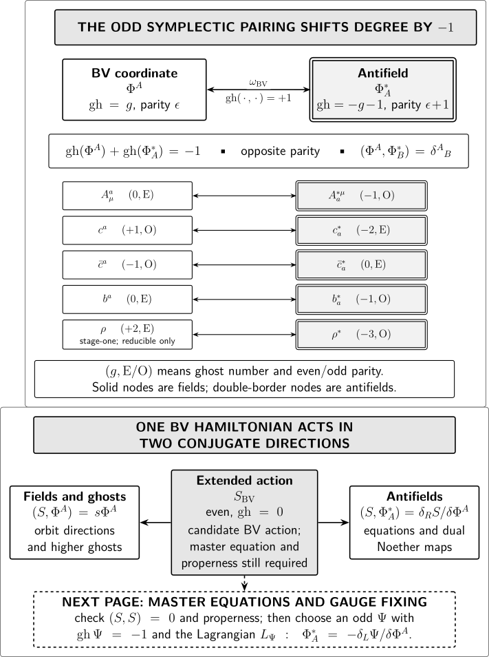
The upper panel records the degree-$-1$ pairing and degree-$+1$ antibracket. The dashed strip is now implemented: first check the master equation and properness, then use an odd $\Psi$ with $\operatorname{gh}\Psi=-1$ to select $\Phi^*=-\delta_L\Psi/\delta\Phi$. The diagram is schematic and does not assert that every global Lagrangian is a graph or that the quantum measure is already defined.

The same construction can be written as a triangular anticanonical change of coordinates. With

$$\operatorname{ad}_G F=(G,F),$$

an odd generator $G$ of ghost number $-1$ preserves parity and ghost number, and the shifted Jacobi identity makes $e^{\operatorname{ad}_G}$ preserve the antibracket. For a field-only $\Psi$,

$$\widehat\Phi^A=\Phi^A, \qquad \widehat\Phi_A^* = \Phi_A^* +\frac{\delta_L\Psi}{\delta\Phi^A}.$$

Thus $\mathcal L_\Psi$ is the zero section $\widehat\Phi^*=0$, and in the passive convention the transformed action is

$$\widehat S=e^{-\operatorname{ad}_\Psi}S.$$

Anticanonical transformations preserve the CME. They do not automatically preserve a chosen density, the BV Laplacian, an integration cycle, or the QME. The required density and Berezinian correction is derived in Gomis, París, and Samuel 1995, § 8.6, arXiv v1, pp. 112–114, eqs. (8.43)–(8.46), Open PDF. That distinction is the quantum content of the next section.

The quantum master equation includes the regulated measure

Start with a finite flat Darboux chart and its translation-compatible density. If $\epsilon_A$ is the parity of $\Phi^A$, define

$$\Delta_0F = \sum_A(-1)^{\epsilon_A} \frac{\partial_L}{\partial\Phi^A} \left( \frac{\partial_LF}{\partial\Phi_A^*} \right).$$

This operator is odd, raises ghost number by one, and satisfies $\Delta_0^2=0$. It is second order rather than a derivation. Its failure to obey the ordinary product rule generates the antibracket:

$$\begin{aligned} \Delta_0(FG)={}&(\Delta_0F)G +(-1)^{\epsilon_F}F\Delta_0G\\ &+(-1)^{\epsilon_F}(F,G). \end{aligned}$$

Equivalently,

$$(F,G) = (-1)^{\epsilon_F} \left[ \Delta_0(FG) -(\Delta_0F)G -(-1)^{\epsilon_F}F\Delta_0G \right].$$

With the present convention $X_FG=(F,G)$, the corresponding divergence translation is $\Delta_0F=-\tfrac12\operatorname{div}_0X_F$. References that define the Hamiltonian vector field in the opposite slot carry the opposite sign.

A nonflat density $\mu$ changes the operator to $\Delta_\mu$. Nilpotency then requires compatibility between the odd symplectic structure and the density. In a continuum field theory the displayed coordinate formula contains coincident functional derivatives. It is therefore only mnemonic until a finite regulator, effective construction, or renormalized composite operator defines $\Delta_\mu$. Antifield-linearity does not by itself justify setting a formal continuum $\Delta S$ to zero. The modern finite-versus-field-theory limitations are summarized in Cattaneo, Mnev, and Schiavina 2025, §§ 4.1 and 4.4, arXiv v1, pp. 10–12, Open PDF.

A recent pAQFT construction obtains a renormalized modified QME for smoothened marked hypersurfaces and studies Abelian Yang–Mills theory, but it assumes Green-hyperbolicity, spacetime cutoffs, and perturbative renormalization. Its Abelian comparison with sharp BV–BFV data further assumes convergent smoothened BV–BFV data. It is frontier evidence, not a general nonperturbative boundary theorem Rejzner and Schiavina 2026, §§ 4.1–4.3 and 5.3, arXiv v1 preprint, pp. 34–44 and 51–56, Open PDF.

For the Lorentzian weight $e^{iS_\hbar/\hbar}$, the quantum master equation (QME) is

$$\boxed{ \mathcal B(S_\hbar) := \frac12(S_\hbar,S_\hbar) -i\hbar\Delta_\mu S_\hbar =0 }.$$

The exponential form is exactly

$$\mathcal B(S_\hbar)=0 \quad\Longleftrightarrow\quad \Delta_\mu e^{iS_\hbar/\hbar}=0.$$

Define the quantum BV differential

$$\sigma_\hbar F = (S_\hbar,F)-i\hbar\Delta_\mu F.$$

When $\Delta_\mu^2=0$, the product identity and Jacobi relation give

$$\sigma_\hbar^2F = \bigl(\mathcal B(S_\hbar),F\bigr), \qquad \sigma_\hbar\mathcal B(S_\hbar)=0.$$

Thus the QME makes $\sigma_\hbar$ nilpotent. If $S_\hbar=S+\hbar S_1+O(\hbar^2)$, the first two orders read

$$\frac12(S,S)=0, \qquad (S,S_1)=i\Delta_\mu S.$$

The second equation asks whether the regulated measure term is removable by an allowed one-loop correction. It is not a declaration that every $\Delta_\mu S$ is an anomaly. The measure, gauge-fermion, and quantum master conditions are developed in Fuster, Henneaux, and Maas 2005, §§ 8–9, arXiv v2, pp. 18–21, especially eqs. (8.6)–(8.18) and (9.1)–(9.4), Open PDF.

The master equations are not the Zinn–Justin equation

Three related identities occur at different stages:

identity	primary object	extra data already chosen
classical master equation	classical extended action $S_{\mathrm{BV}}$	odd field–antifield geometry and a proper classical resolution
quantum master equation	regulated or renormalized quantum action $S_\hbar$	density, $\Delta_\mu$, counterterms, and an integration prescription
Zinn–Justin equation	renormalized 1PI functional $\Gamma$	gauge fixing, nonlinear-composite sources, Legendre transform, and subtraction scheme

In the partial shifted chart of Slavnov–Taylor and Zinn–Justin Identities, the minimal antifields correspond to the external sources as $A^*=K$ and $c^*=-L$ in this chapter’s sign convention. That bridge does not identify $S_{\mathrm{BV}}$ with $\Gamma$: the latter is built from mean fields after gauge fixing and quantum renormalization. The CME, QME, and Zinn–Justin equation therefore constrain related constructions, not three names for one functional equation.

Quantum observables descend only under BV Stokes hypotheses

A classical BV observable of ghost number zero obeys

$$(S,\mathcal O)=0, \qquad \mathcal O\sim\mathcal O+(S,X), \quad \operatorname{gh}X=-1.$$

At the quantum level the corresponding equations are

$$\sigma_\hbar\mathcal O=0, \qquad \mathcal O\sim\mathcal O+\sigma_\hbar X.$$

The antifield expansion of $\mathcal O$ supplies a descent through gauge variation, equations of motion, and higher relations. Its lowest antifield-independent component is an on-shell gauge-invariant observable candidate. This functional cohomology is not automatically state cohomology, and a local density modulo spacetime total derivatives belongs to the different complex $H(s\mid d)$.

For a local ghost-number-zero top form, the first observable-descent equation is

$$sa_d^0+\mathrm d a_{d-1}^1=0.$$

On a manifold with boundary it gives

$$s\int_Ma_d^0 = -\int_{\partial M}a_{d-1}^1.$$

Thus even a class that closes modulo a spacetime derivative needs a boundary cancellation, boundary observable, or flux condition before its integral is BRST closed.

Under the QME,

$$\Delta_\mu \left( \mathcal Oe^{iS_\hbar/\hbar} \right) = \frac{i}{\hbar} (\sigma_\hbar\mathcal O) e^{iS_\hbar/\hbar}.$$

Likewise, a quantum-exact insertion satisfies

$$(\sigma_\hbar X)e^{iS_\hbar/\hbar} = -i\hbar\Delta_\mu \left( Xe^{iS_\hbar/\hbar} \right).$$

It decouples only if the integral of the right-hand side vanishes. At a finite regulator, BV Stokes gives that conclusion for a compatible density and an admissible Lagrangian cycle with no boundary or contour flux. The underlying finite-dimensional deformation theorem is Schwarz 1993, pp. 2–4, eqs. (6)–(9), arXiv v1, Open PDF; it is not by itself a continuum functional-integral theorem.

Let $\Psi_t$ be an admissible family that remains in the same integration class. Schematically, after transforming the observable with the gauge choice,

$$\frac{\mathrm d}{\mathrm dt}Z_{\Psi_t} = \int_{\mathcal L_{\Psi_t}} \Delta_\mu \left( \dot\Psi_t e^{iS_\hbar/\hbar} \right) =0.$$

The equality needs all of the following:

• a compatible $\mu$ and $\Delta_\mu$ with $\Delta_\mu^2=0$;
• a proper QME solution and a quantum-closed insertion;
• an admissible family of cycles with no boundary-at-infinity or contour flux;
• no untreated zero mode, stabilizer, determinant-rank jump, or Gribov horizon crossed by the family;
• boundary conditions preserved by the Hamiltonian flow; and
• a regulator removal and renormalization prescription that preserves the identity.

Therefore gauge independence means equality of the resulting quantum observables or normalized correlators under the stated transport. It does not mean equality of the gauge-fixed integrands, equality of arbitrary off-shell Green functions, or equivalence across a singular or globally disconnected gauge-fixing cycle.

An anticanonical transformation illustrates the same distinction. It preserves the bracket and CME. In the passive convention, the infinitesimal QME-compatible change of the action contains the measure correction

$$\delta_GS_\hbar = \sigma_\hbar G = (S_\hbar,G)-i\hbar\Delta_\mu G.$$

For a field-only triangular shift in a finite flat chart, $\Delta_0\Psi=0$. A general bracket-canonical map need not be unimodular, so its density and Jacobian must still be transported.

A QME residual is a candidate anomaly obstruction

Suppose a regulated, local perturbative construction solves the QME through order $\hbar^{n-1}$ but leaves

$$\mathcal B(S_\hbar) = \hbar^n\mathcal A_n +O(\hbar^{n+1}).$$

The identity $\sigma_\hbar\mathcal B=0$ implies at the first nonzero order

$$(S,\mathcal A_n)=0, \qquad \operatorname{gh}\mathcal A_n=1.$$

If $\mathcal A_n=(S,\mathcal C_n)$ for an allowed local, even, ghost-number-zero counterterm, shifting $S_\hbar\mapsto S_\hbar-\hbar^n\mathcal C_n$ removes that breaking at the order shown. A nontrivial class is a candidate anomaly obstruction. It becomes a realized anomaly only after locality, power counting, subsidiary identities, regulator dependence, and its coefficient have been established. The local ghost-number-one classification and its counterterm ceiling are given in Barnich, Brandt, and Henneaux 2000, § 2.6 and § 12.3, arXiv v3, p. 16 and pp. 119–121, eqs. (2.32)–(2.38) and (12.7), Open PDF.

For a local ghost-number-one anomaly density on a $d$-manifold, the consistency descent begins

$$sa_d^1+\mathrm d a_{d-1}^2=0.$$

On a manifold with boundary,

$$s\int_Ma_d^1 = -\int_{\partial M}a_{d-1}^2.$$

Thus a spacetime-exact term is not automatically trivial. Boundary counterterms, boundary fields, or a flux condition must cancel the surface term. The local test also does not classify large-gauge or other global anomalies.

Bounded Maxwell checks the master and gauge-fixing signs at finite rank

Let $\Sigma$ be a smooth bounded connected spatial region and work on a cylinder $I\times\Sigma$. Use the based identity-component redundancy group, so the gauge parameter and ghost have Dirichlet trace on $\partial\Sigma$. Choose temporal endpoint data and remaining boundary data that make the Maxwell action differentiable. As on the prerequisite page, take a finite, BRST-stable Galerkin core: retain smooth Dirichlet scalar modes, their exact one-form gauge directions, compatible transverse modes, and independent nonminimal spaces.

Write the retained BRST rules as

$$sA^r=R^r{}_{\alpha}c^\alpha, \qquad sc^\alpha=0, \qquad s\bar c^\alpha=b^\alpha, \qquad sb^\alpha=0,$$

where $R^r{}_{\alpha}$ is constant. Let $S_{0,N}$ be the gauge-invariant finite Maxwell action, and define

$$S_N = S_{0,N} +A_r^*R^r{}_{\alpha}c^\alpha -\bar c_\alpha^*b^\alpha.$$

Gauge invariance is the finite Noether identity

$$\frac{\partial S_{0,N}}{\partial A^r} R^r{}_{\alpha}=0.$$

The entire classical master residual is therefore

$$\frac12(S_N,S_N) = \frac{\partial S_{0,N}}{\partial A^r} R^r{}_{\alpha}c^\alpha =0.$$

For the finite flat density, direct differentiation also gives

$$\Delta_0S_N=0.$$

The reason is concrete: $S_{0,N}$ has no antifields, $A_r^*R^r{}_{\alpha}c^\alpha$ has no $A^r$ dependence, and $-\bar c_\alpha^*b^\alpha$ has no $\bar c^\alpha$ dependence. Hence $S_N$ satisfies the finite QME with no loop correction. This is an exact regulated algebraic check, not a claim that the unregulated Maxwell functional Laplacian exists.

Properness is a separate finite-core hypothesis. After the based boundary condition removes constant stabilizers, require $R^r{}_{\alpha}$ to have full column rank and require the kernel of the Hessian of $S_{0,N}$ on the declared core to be exactly the retained gauge image, with physical, harmonic, and temporal zero modes treated separately. If either rank condition fails, the field–antifield resolution or zero-mode treatment must be repaired before a gauge-fixing graph is used. Neither $\Delta_0S_N=0$ nor the later Dirichlet FP gap proves this properness condition.

Now choose a linear gauge condition

$$F_N^\alpha(A)=F^\alpha{}_rA^r, \qquad M^\alpha{}_{\beta} = F^\alpha{}_rR^r{}_{\beta},$$

and the gauge-fixing fermion

$$\Psi_N = \bar c_\alpha \left( F_N^\alpha(A)+\frac\xi2b^\alpha \right).$$

The graph equations are

$$\begin{aligned} A_r^*&=-\bar c_\alpha F^\alpha{}_r, & c_\alpha^*&=0,\\ \bar c_\alpha^*&=-\left(F_N^\alpha+\frac\xi2b^\alpha\right), & b_\alpha^*&=-\frac\xi2\bar c_\alpha. \end{aligned}$$

Substitution into $S_N$ gives

$$\begin{aligned} S_{\Psi,N}={}&S_{0,N} +b_\alpha F_N^\alpha +\frac\xi2b_\alpha b^\alpha\\ &-\bar c_\alpha M^\alpha{}_{\beta}c^\beta. \end{aligned}$$

This reproduces the chapter’s minus sign in the ghost action without an integration by parts. It is also the direct finite identity $S_{\Psi,N}=S_{0,N}+s\Psi_N$.

For Coulomb gauge, $F[A]=\partial_iA_i$ and

$$M_0=\Delta_D$$

on $H^2(\Sigma)\cap H_0^1(\Sigma)$, while the positive spectral operator is $-\Delta_D$. The ghost remains in the based Dirichlet domain; $\bar c$, $b$, and the antifields occupy separately declared output and dual spaces and do not inherit that trace condition. At $\xi=0$, $b$ imposes $F=0$ sharply. For $\xi\ne0$, its equation is $F+\xi b=0$, and eliminating it yields the longitudinal term $-F^2/(2\xi)$.

Changing $\xi$ changes both the Lagrangian graph and the off-shell action:

$$\frac{\partial\Psi_N}{\partial\xi} = \frac12\bar c_\alpha b^\alpha, \qquad \frac{\partial S_{\Psi,N}}{\partial\xi} = \frac12b_\alpha b^\alpha.$$

Only the BV-Stokes argument licenses independence of transported quantum-closed observables.

The three readings are now explicit:

reading	bounded Maxwell statement
Orbit	$c
Charge	Boundary-nontrivial transformations and possible surface charges are absent from this ghost complex; gauge fixing and antifields do not make them exact.
Gauge fixed	$\mathcal L_{\Psi_N}$ produces the Coulomb condition, the $b$ equation, and the Dirichlet ghost operator; its local usefulness still requires the FP gap and an admissible contour.

The charge statement depends on the boundary phase-space setup. It is supported for field-independent transformations by Assanioussi et al. 2024, §§ 3.1–3.3, arXiv v2, pp. 13–16, eqs. (3.24)–(3.26), Open PDF. If boundary fields are retained rather than excluded by boundary conditions, the bulk data must be enlarged to BV–BFV data; a current review emphasizes that boundary conditions and the regularized BV Laplacian remain separate parts of quantization Cattaneo, Mnev, and Schiavina 2025, §§ 4.4 and 4.6, arXiv v1, pp. 12–14, Open PDF.

For compact Yang–Mills theory the same fermion gives $M_A=\partial_iD_i$ on the smooth based core, while $sc$ and the minimal BV action are nonlinear. The construction remains local to an FP-invertible patch. A Gribov horizon or a nonperturbative restriction of the integration domain can invalidate the cycle-deformation argument without invalidating the local algebraic CME. The separation between zero modes, the first region, and remaining copies is reviewed in Vandersickel and Zwanziger 2012, §§ 2.2–2.2.1, arXiv v2, pp. 20–25, Open PDF.

What the master equations do—and do not—imply

premise	licensed conclusion	conclusion that does not follow
complete odd field–antifield pairing	a nondegenerate antibracket on the declared domain	a density, BV Laplacian, or gauge choice
$\tfrac12(S,S)=0$	nilpotent classical Hamiltonian differential	properness, QME, or gauge independence
field-only, differentiable, domain-admissible odd $\Psi$ with ghost number $-1$	a local Lagrangian graph	transversality, a global slice, or a convergent contour
anticanonical transformation	preservation of the antibracket and CME	preservation of the density, $\Delta_\mu$, or QME
QME plus BV Stokes and an admissible cycle deformation	gauge-choice invariance of transported quantum-closed quantities	equality of arbitrary off-shell correlators
$\sigma_\hbar\mathcal A=0$ at ghost number one	a consistency condition on a candidate breaking	a nonzero anomaly coefficient or a global anomaly
a BRST-stable bulk boundary domain	a bulk master identity for the declared redundancies	vanishing of every boundary charge or flux

The common thread is that algebra, measure, integration cycle, and global quotient are different layers. BV relates them; it does not collapse them into one assumption.

Common pitfalls

Treating the CME as automatic. The antibracket is odd, so the shifted antisymmetry does not force $(S,S)$ to vanish for even $S$. The CME is the nontrivial condition that makes the Hamiltonian vector field nilpotent.

Replacing properness by the master equation. A solution can satisfy the CME while omitting a generator, reducibility relation, or compatible dual direction. Properness and boundary completeness must be checked separately.

Calling every odd functional a gauge fermion. The fermion must also have ghost number $-1$, preserve the declared domain, and define an admissible Lagrangian graph. A singular graph is not repaired by its parity.

Writing a continuum $\Delta S$ as though it were finite. The BV Laplacian contains coincident functional derivatives and depends on a density. A regulator or renormalized construction must define it before the QME is an equation.

Assuming canonical means quantum-equivalent. An anticanonical map preserves the bracket. Quantum equivalence additionally transports the density, Jacobian, cycle, insertions, boundary data, and counterterms.

Using BV Stokes across a singular slice. Zero modes, determinant-rank jumps, a Gribov horizon, or boundary flux can invalidate the integration-by- parts step. Algebraic nilpotency may remain perfectly intact.

Calling every closed ghost-number-one residual an anomaly. Closure is the consistency condition. A realized anomaly also needs a nonremovable class and a nonzero regulated quantum coefficient.

Check your understanding

Runnable companion. No interactive BRST–BV calculation is currently available, so the finite grading, sign, and master-residual checks are worked explicitly here.

These checks are not registered exercises, checkpoints, or capstones.

1. Recover the QME from the exponential. Starting from the second-order product rule, compute $\Delta_\mu e^{iS_\hbar/\hbar}$.

Solution

For even $S_\hbar$,

$$\Delta_\mu e^{iS_\hbar/\hbar} = \left[ \frac{i}{\hbar}\Delta_\mu S_\hbar -\frac{1}{2\hbar^2}(S_\hbar,S_\hbar) \right] e^{iS_\hbar/\hbar}.$$

Multiplying the coefficient by $-\hbar^2$ gives $\tfrac12(S_\hbar,S_\hbar)-i\hbar\Delta_\mu S_\hbar$. Thus the exponential is $\Delta_\mu$-closed exactly when the QME holds.

2. Check the Maxwell master residual. Evaluate $\tfrac12(S_N,S_N)$ and $\Delta_0S_N$ directly.

Solution

Only the bracket of $S_{0,N}$ with $A_r^*R^r{}_{\alpha}c^\alpha$ survives, so

$$\frac12(S_N,S_N) = \frac{\partial S_{0,N}}{\partial A^r} R^r{}_{\alpha}c^\alpha =0$$

by the Noether identity. Each antifield term is independent of its paired field, so its $\Delta_0$ contraction vanishes; $S_{0,N}$ has no antifields. Therefore $\Delta_0S_N=0$.

3. Derive the gauge-fixed signs. Substitute the four graph equations from $\Psi_N$ into $S_N$.

Solution

The minimal antifield term becomes

$$A_r^*R^r{}_{\beta}c^\beta = -\bar c_\alpha F^\alpha{}_rR^r{}_{\beta}c^\beta = -\bar c_\alpha M^\alpha{}_{\beta}c^\beta.$$

The nonminimal term gives

$$-\bar c_\alpha^*b^\alpha = b_\alpha F_N^\alpha +\frac\xi2b_\alpha b^\alpha.$$

Together they reproduce $S_{0,N}+s\Psi_N$ with the required minus ghost term.

4. Diagnose a removable quantum breaking. Suppose the first residual is $\hbar^n\mathcal A_n$ with $\mathcal A_n=(S,\mathcal C_n)$. Which counterterm removes it at that order?

Solution

Use

$$S_\hbar\longmapsto S_\hbar-\hbar^n\mathcal C_n.$$

The linearized change of the master residual is $-\hbar^n(S,\mathcal C_n)=-\hbar^n\mathcal A_n$, so it cancels the first breaking. The counterterm is admissible only if it also satisfies locality, power counting, boundary, and subsidiary-identity requirements.

5. Test the gauge-parameter claim. Why does $\partial_\xi S_{\Psi,N}=s(\bar c_\alpha b^\alpha/2)$ not by itself prove $\xi$-independence of a quantum observable?

Solution

The equation is a classical exactness statement. Turning it into a vanishing derivative of an expectation value additionally requires a QME-compatible measure and BV Laplacian, a quantum-closed insertion transported with the gauge choice, an admissible family of integration cycles, no boundary or contour flux, and a regulator/renormalization prescription that preserves the identity. Stabilizers, residual zero modes, determinant-rank jumps, or a Gribov horizon can invalidate the cycle deformation even while the displayed BRST identity remains true.

Where the construction continues

What Is an Anomaly? separates removable quantum breakings from genuine local and global obstructions. The BV Complex and the Classical Master Equation develops the theorem-level homological construction, while Quantum Master Equation and Anomaly Obstructions develops renormalized obstruction theory. BV–BFV Structures, Boundaries, and Gluing handles surviving boundary fields and the modified master identity. Gauge Theories and the Standard Model supplies model-specific Yang–Mills loop calculations. Gauge, BRST, and BV Interfaces on Curved Backgrounds adds local covariance, causal renormalization, and gravitational or curved- background domains.

References

• Assanioussi, Mehdi, Jerzy Kowalski-Glikman, Ilkka Mäkinen, and Ludovic Varrin. “On the Covariant Formulation of Gauge Theories with Boundaries.” Classical and Quantum Gravity 41, no. 11 (2024): 115007. DOI. Open PDF, arXiv v2.
• Barnich, Glenn, Friedemann Brandt, and Marc Henneaux. “Local BRST Cohomology in Gauge Theories.” Physics Reports 338, no. 5 (2000): 439–569. DOI. Open PDF, arXiv v3.
• Batalin, I. A., and G. A. Vilkovisky. “Gauge Algebra and Quantization.” Physics Letters B 102, no. 1 (1981): 27–31. DOI.
• Cattaneo, Alberto S., Pavel Mnev, and Nicolai Reshetikhin. “Classical BV Theories on Manifolds with Boundary.” Communications in Mathematical Physics 332, no. 2 (2014): 535–603. DOI. Open PDF, arXiv v3.
• Cattaneo, Alberto S., Pavel Mnev, and Michele Schiavina. “BV Quantization.” In Encyclopedia of Mathematical Physics, 2nd ed., edited by Richard J. Szabo and Martin Bojowald, vol. 5, 543–555. Oxford: Elsevier, 2025. DOI. Open PDF, arXiv v1.
• Fuster, Andrea, Marc Henneaux, and Axel Maas. “BRST-Antifield Quantization: A Short Review.” International Journal of Geometric Methods in Modern Physics 2, no. 5 (2005): 939–964. DOI. Open PDF, arXiv v2.
• Gomis, Joaquim, Jordi París, and Stuart Samuel. “Antibracket, Antifields and Gauge-Theory Quantization.” Physics Reports 259, nos. 1–2 (1995): 1–145. DOI. Open PDF, arXiv v1.
• Rejzner, Kasia, and Michele Schiavina. “Perturbative Algebraic Quantum Field Theory with Smoothened Boundary.” arXiv preprint arXiv:2607.13765v1 (2026). Abstract. Open PDF.
• Schwarz, Albert. “Geometry of Batalin–Vilkovisky Quantization.” Communications in Mathematical Physics 155, no. 2 (1993): 249–260. DOI. Open PDF, arXiv v1.
• Vandersickel, Nele, and Daniel Zwanziger. “The Gribov Problem and QCD Dynamics.” Physics Reports 520, no. 4 (2012): 175–251. DOI. Open PDF, arXiv v2.