

Local Potentials and Global Gauge Configurations
A global gauge configuration is a bundle with a connection, not one potential that must be smooth in every coordinate patch. On an open cover it is encoded by local potentials and transition functions satisfying overlap and cocycle conditions. Nontrivial transition data can obstruct a single global potential and, for compact , can carry quantized magnetic flux. The local field equations alone do not decide which bundle sectors enter the theory. This page develops the smooth patchwise description, its global observables, and the Dirac-monopole flux sector; classification theorems, differential cohomology, and monopole-core dynamics remain outside its scope.
Required background. Gauge Fields, Redundancy, and Observable Content supplies the local finite gauge law and the distinction between admissible transformations and redundancy. Vector, Principal, and Associated Bundles supplies principal bundles, local sections, and transition functions.
Helpful background. Characteristic Classes and Chern–Weil Theory supplies the general characteristic-class interpretation, while Homotopy, Degree, Winding, and Covering Spaces supplies the winding number used in the compact- example.
A global connection is compatible patch data
Section titled “A global connection is compatible patch data”Let be a principal bundle with compact structure group , and choose an open cover . In a representation of , write the local matter representatives and transition functions so that on an overlap
Consistency on double and triple overlaps requires
The second equation is the cocycle condition. It says that transporting a local frame around a triple overlap returns to the same frame. Subject to the usual regularity assumptions, such transition data reconstruct a bundle; changing the data by compatible local frame changes gives an isomorphic presentation rather than a new local force law.
Let be the Hermitian local potential on , with for one simple or factor. Requiring fixes the overlap law:
where
The inhomogeneous term is precisely what makes the covariant derivatives agree. The curvature patches homogeneously, so the collection is a global section of . In Abelian theory the conjugations disappear and the agree as one ordinary global two-form.
Nakahara states the cocycle conditions, reconstructs bundles from valid transition data, and derives the local connection compatibility law in Nakahara 2003, 2nd ed., § 9.2.1, p. 351; § 9.2.2, pp. 353–354; and § 10.1.3, pp. 377–380. His connection forms are geometrically normalized and may be anti-Hermitian; the equations above translate them to the site’s Hermitian convention.
A connection itself is global on the total space . What can fail to exist is a global section with which to pull it back to one Lie-algebra-valued potential on the base. A nontrivial bundle still has local potentials on a sufficiently fine cover.
Local frame changes and gauge transformations
Section titled “Local frame changes and gauge transformations”Redefine the local representatives by , with . To describe the same global bundle and connection, the other local data must change simultaneously:
The cocycle condition and curvature patching are unchanged. This simultaneous change of and is a change of local description of the same global connection.
A nonidentity transition function by itself therefore does not prove that a bundle is nontrivial. If the full cocycle can be removed by such local redefinitions, it is a presentation of a trivial bundle. The obstruction is the impossibility of removing all transition data compatibly, not the mere appearance of an in one chosen cover.
An active gauge transformation of a fixed bundle presentation is instead a compatible collection satisfying
on every overlap. It acts on each by the same inhomogeneous local law. Whether that active transformation is quotiented also depends on the boundary conditions and its complete generator, as established on Gauge Orbits, Gauss Constraints, and Stabilizers. Neither a frame change nor a smooth bundle automorphism changes the bundle’s topological sector.
This distinction prevents a common confusion. A transition function has the same algebraic form as a finite local gauge transformation, but it relates two descriptions on an overlap. It need not extend to one globally defined map on , and its failure to do so can be the information that makes the bundle nontrivial.
Curvature and holonomy assemble globally
Section titled “Curvature and holonomy assemble globally”Gauge-invariant polynomials in the curvature agree across overlaps. For example, the matrix-valued changes by conjugation, while traces such as agree exactly. In compact , the normalized periods of the global two-form can label flux sectors.
Parallel transport also assembles from local data. When a path crosses from to , the transition matrix identifies the two local fibers; the ordered product of local transporters and transition matrices is independent of where the cover was subdivided. For a closed curve based at , the holonomy changes only by conjugation at , so
is independent of the local frame. Tong derives the endpoint transformation and traced closed holonomy in Tong 2018, § 2.1.3, pp. 33–34, official full-notes PDF. The allowed representation is part of the global theory specification, not something fixed by the Lie algebra alone.
Curvature and holonomy contain different information. A flat connection can have nontrivial holonomy around a noncontractible cycle, while a nonzero local curvature need not imply a nontrivial bundle. It is a nonzero characteristic period, not merely somewhere, that obstructs a global trivialization in the Abelian example below.
Even curvature periods have a limit: they detect the image of the first Chern class in real cohomology. Torsion bundle data has zero de Rham image and can be invisible to ; its treatment requires holonomy or a differential cohomological refinement beyond this page.
Compact U(1) flux from two smooth potentials
Section titled “Compact U(1) flux from two smooth potentials”Take compact and choose the generator and field normalization so that a unit-weight field carries the smallest positive faithful electric charge and transforms as . Cover a sphere by northern and southern patches and , and orient it by . Reversing this orientation sends the displayed sector label to . For an integer , define
is regular at the north pole and at the south pole. On their overlap,
Although shifts when , the transition function is single-valued exactly when . Both local potentials give the same smooth curvature,
and hence
This is the first Chern number in the chosen charge normalization. For , one nonsingular global potential on cannot exist: if globally, Stokes’ theorem on the closed sphere would give . The two regular potentials do not hide a physical string; they are the correct local representatives of a smooth connection on a nontrivial bundle.
The diagram below collects the full patch calculation. Read the top row as three descriptions on one cover, not as three physical regions: the dashed middle box is the overlap relation that glues the two regular potentials. Every downward arrow reaches the same curvature and the same oriented flux.
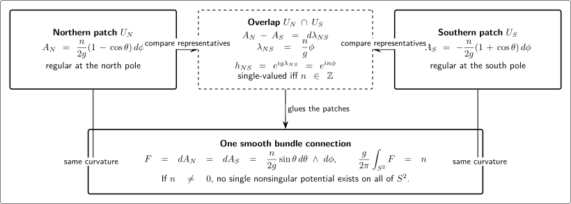
Two regular compact- potentials on differ on their overlap by , with single-valued transition function exactly for . They produce the same curvature and normalized flux . The figure is schematic and not to scale; for it is the single global base potential—not the smooth bundle connection—that fails to exist.
Tong gives the physical patch construction and Dirac quantization argument in Tong 2018, § 1.1.2, pp. 6–8, official full-notes PDF. Nakahara gives the corresponding bundle and flux calculation in Nakahara 2003, 2nd ed., § 10.5.2, pp. 400–401. Both sources place charge factors differently; the integer period is invariant under the translation to the displayed convention.
Compactness and the charge spectrum are essential. The Lie algebra by itself does not impose this integer, and a theory with additive gauge group instead has transition maps into , whose fundamental group is trivial. If the smallest faithful charge is normalized differently, the explicit flux unit changes with it. Global Form, Matter Representations, and the Faithful Gauge Group develops that dependence.
A bounded Maxwell sector in three descriptions
Section titled “A bounded Maxwell sector in three descriptions”Let the spatial region be a spherical shell . The monopole core is excluded, and the angular patch data above extend across the shell. The Bianchi identity gives inside , while the two oriented boundary fluxes cancel in their sum. Their common unsigned flux can nevertheless be nonzero and carry the sector label . If the inner ball contains an external magnetic defect, this flux is interpreted as its magnetic charge; the page does not construct a dynamical or finite-energy monopole core.
The same configuration can be organized in three complementary languages.
Patch/orbit description. Within the chosen bundle , quotient compatible local potentials by the zero-generator subgroup selected by the boundary conditions. What remains is the global connection orbit in the fixed sector ; admissible boundary transformations with nonzero generators act as physical symmetries rather than redundancies.
Flux/sector description. Integrate the global curvature over a boundary sphere. This extracts the integer magnetic sector; electric Gauss charges remain a separate boundary question.
Gauge-fixed description. Impose a condition such as Coulomb gauge on compatible local representatives. The result is a calculational representative; it does not remove the winding of .
A patchwise gauge condition must respect the overlap law. For , no smooth gauge choice can set everywhere and replace by one nonsingular global potential. Forcing such a representative produces a Dirac string singularity; it does not prove that the smooth bundle connection was singular. Gauge fixing works within a sector and does not choose the sector.
Magnetic flux is also distinct from the electric surface generator discussed on the preceding pages. Which boundary transformations are quotiented depends on the action boundary terms, boundary conditions, and allowed fields. Harlow and Wu explain why those data define the boundary theory in Harlow and Wu 2020, § 1, pp. 3–4, JHEP PDF. The local Maxwell equations and the integer patch data do not settle that electric charge question.
Local equations do not select the sector sum
Section titled “Local equations do not select the sector sum”The Maxwell equations can be written in every patch and glued covariantly, but they do not say whether a compact- problem fixes one flux sector or sums over several. Schematically, one may define
Here denotes a bundle in flux sector , is the set of sectors admitted by the problem, and is the same subgroup of admissible transformations whose canonical generators vanish on the allowed configurations. The factors may encode additional global or topological data. This notation is only schematic. Boundary conditions can fix flux, defects can prescribe it, and a theory definition can restrict or weight sectors. None of those choices follows from the local expression alone. In a general compact Yang–Mills theory, the analogous sum is indexed by the allowed bundle classes , not necessarily by one integer.
The full classification of bundles and differential refinements belongs to the prerequisite mathematics and to Gauge Configuration Groupoids and Moduli. Smooth monopole solutions and their dynamics belong to Monopoles and Dyons.
Common pitfalls
Section titled “Common pitfalls”Calling the connection only a local object. The connection is global on the principal bundle. The potentials are its local representatives on the base.
Treating a transition function as one global gauge transformation. It is defined on an overlap and may have winding that cannot be extended away. That failure can encode the bundle sector.
Calling every nonidentity transition function topological. A removable cocycle can contain nonidentity functions in a poor choice of local frames. Nontriviality is the obstruction to eliminating the complete transition data by compatible local redefinitions.
Inferring nontrivial topology from nonzero curvature at one point. A trivial bundle can support curved connections. In compact , the normalized integral period is the relevant obstruction in this example.
Assuming the Lie algebra quantizes flux. Compact global form and the faithful charge spectrum fix the integer normalization. Replacing by changes the conclusion.
Using gauge fixing to erase a flux sector. Gauge fixing selects local representatives within an orbit. It cannot turn a nonzero first Chern number into zero.
Reading the patch construction as monopole dynamics. It describes a smooth bundle outside an excluded core or defect. It does not establish a finite-energy monopole solution.
Check your understanding
Section titled “Check your understanding”- Starting from , derive the overlap law for and show that . Explain why the cocycle condition is required on a triple overlap.
- For the northern and southern compact- potentials, compute the transition function, curvature, and normalized flux. Why does a nonzero answer rule out one smooth global potential on but not a smooth global connection on the bundle?
Solution
Requiring gives
Equating the terms multiplying yields
Since and on the overlap, squaring the operators gives . On a triple overlap, the principal-bundle transition functions satisfy by definition. Successive substitutions give in a representation ; a faithful representation independently detects the group-valued cocycle, whereas nonfaithful matter sees it only modulo .
For the monopole patches,
so and . Single-valuedness around the equator requires . Differentiation gives
and direct integration gives
If one global base potential existed, would be exact and Stokes’ theorem would force this integral to vanish. The global bundle connection does exist: its two local pullbacks are , joined by the valid transition function.
What to carry forward
Section titled “What to carry forward”Gauge-Invariant and Dressed Observables uses Wilson lines and dressings to construct quantities on the physical quotient. Global Form, Matter Representations, and the Faithful Gauge Group determines which transition functions and representations define the actual group, and Large Gauge Transformations and Topological Sectors separates bundle sectors from disconnected transformations within a sector. The allowed electric and magnetic line spectrum is completed at Genuine Line Spectra, Discrete Theta Data, and Theory Specification.
References
Section titled “References”- Harlow, Daniel, and Jie-qiang Wu. “Covariant Phase Space with Boundaries.” Journal of High Energy Physics 10 (2020): 146. DOI. Open PDF
- Nakahara, Mikio. Geometry, Topology and Physics. Second edition. Bristol: Institute of Physics Publishing, 2003. Publisher page
- Tong, David. Gauge Theory. Cambridge Part III Mathematical Tripos lecture notes, 2018. Official course page. Official PDF