Boundaries, Flux, and Boundary Ward Identities

Allowing a localized symmetry parameter to reach a physical boundary does not change the Ward–Takahashi identity in the interior. It does expose a second, boundary-supported identity. The normal component of the bulk current, the divergence of any boundary current, variations of boundary operators or sources, and a possible regulated Jacobian must then balance one another.

Consequently, local bulk conservation does not by itself make a bulk charge independent of the hypersurface on which it is measured. Positive outward flux lowers the bulk charge. If boundary degrees of freedom absorb that flux, their charge can rise by the same amount and the combined charge can remain conserved. If fixed boundary data are not invariant, the transformation may instead relate different boundary problems rather than give an identity within one theory.

This page treats regulated ordinary continuous symmetries on a finite Lorentzian region. It derives local bulk and wall identities, their integrated balance laws, and a complex-scalar example. Differentiable gauge generators, Hamiltonian surface charges, asymptotic limits, and the classification of quantum anomalies are explicit continuations rather than assumptions here.

Required background. Localized Transformations and Ward–Takahashi Identities fixes the regulated change-of-variables and contact-term conventions. Differential Forms, Integration, Orientation, and Stokes Theorem supplies the outward-first orientation and flux form of Stokes’ theorem.

Helpful background. Contact Terms, Equal-Time Commutators, and Schwinger Terms develops the distributional contacts from the operator side. Classical Symmetries, Currents, and Stress Tensors works representative variational currents and their improvement qualifications.

Localized variations on a bounded region

Let $M_{12}$ be a piecewise-smooth spacetime slab with boundary

$$\partial M_{12} =\Sigma_2\cup(-\Sigma_1)\cup B_{12}.$$

The spacelike caps $\Sigma_1$ and $\Sigma_2$ are given their future-directed orientation when defining charge. The timelike wall $B_{12}$ has outward spacelike normal $n_\mu$, and its spacelike cuts are $S_i=\Sigma_i\cap B_{12}$. Capital indices $A,B,\ldots$ are tangent to the wall; lower-case $a,b,\ldots$ label symmetry generators. We use the site metric and Lorentzian path-integral conventions, and the induced wall measure is $\mathrm d^{d-1}y\sqrt{|\gamma|}$.

Work first at a finite regulator scale $\Lambda$. The state, regulator, integration cycle, boundary action, boundary conditions, and admitted variations are part of the definition of the path integral. Choose the smooth parameter $\alpha^a(x)$ to vanish near the temporal caps but permit it to be arbitrary on the interior of $B_{12}$. This support choice removes cap and corner terms from the local derivation without suppressing the physical wall term that the page is meant to determine.

Retain the current and breaking convention of the prerequisite page:

$$\begin{aligned} \delta_\alpha S_M ={}&- \int_{M_{12}}\!\mathrm d^d x\sqrt{-g}\, j_a^\mu\nabla_\mu\alpha^a \\ &+ \int_{M_{12}}\!\mathrm d^d x\sqrt{-g}\, \alpha^a\mathcal B_a. \end{aligned}$$

Here $\mathcal B_a$ is the bulk explicit-breaking insertion; it vanishes for an exact regulated symmetry. If the wall supports fields or a boundary action, write its localized variation as

$$\begin{aligned} \delta_\alpha S_B ={}&- \int_{B_{12}}\!\mathrm d^{d-1}y\sqrt{|\gamma|}\, k_a^A D_A\alpha^a \\ &+ \int_{B_{12}}\!\mathrm d^{d-1}y\sqrt{|\gamma|}\, \alpha^a\mathcal B_{\partial a}. \end{aligned}$$

The tangential current $k_a^A$ is a boundary Ward current. The insertion $\mathcal B_{\partial a}$ records a noninvariant boundary interaction or fixed boundary source. It is not the surface charge-variation form that appears in the Hamiltonian treatment later in the chapter.

Integrating by parts gives

$$\begin{aligned} \delta_\alpha(S_M+S_B) ={}& \int_{M_{12}}\!\mathrm d^d x\sqrt{-g}\, \alpha^a \bigl(\nabla_\mu j_a^\mu+\mathcal B_a\bigr) \\ &+ \int_{B_{12}}\!\mathrm d^{d-1}y\sqrt{|\gamma|}\, \alpha^a \bigl( D_Ak_a^A-n_\mu j_a^\mu+\mathcal B_{\partial a} \bigr). \end{aligned}$$

The sign of $-n_\mu j_a^\mu$ is fixed: it comes from applying Stokes’ theorem to the minus sign in $-j_a^\mu\nabla_\mu\alpha^a$. Had $\alpha$ reached $S_1$ or $S_2$, integrating the boundary-current term would also have produced a boundary-of-boundary contribution. Boundary conditions as part of the theory, a bulk-plus-boundary action, and a complete first variation are treated systematically in Harlow and Wu 2020, § 1, pp. 3–5, and § 2.2, pp. 11–14, Open PDF.

Setting $\alpha|_{B_{12}}=0$ would recover only the interior relation. It would not prove that the wall coefficient vanishes. The boundary-free regulated change-of-variables calculation is given in Schwartz 2014, § 14.8.1, pp. 278–279; the wall term above is the additional calculation required here.

The interior and wall Ward identities

Let

$$\mathcal X=\prod_{r=1}^{n}\mathcal O_r(x_r), \qquad \mathcal Y=\prod_{s=1}^{m}\widehat{\mathcal O}_s(y_s)$$

contain regulated bulk and wall insertions, respectively. Use

$$U(\epsilon)=e^{-i\epsilon^aQ_a}, \qquad \delta_a\mathcal O=-i[Q_a,\mathcal O].$$

For insertions whose localized transformations contain no derivatives of $\alpha$, define the two contact distributions

$$\begin{aligned} \mathcal C_{M,a}(x;\mathcal X,\mathcal Y) ={}&i\sum_{r=1}^{n}\delta_M(x,x_r) \left\langle \mathrm T\{\mathcal X_{a,r}\mathcal Y\} \right\rangle, \\ \mathcal C_{\partial,a}(y;\mathcal X,\mathcal Y) ={}&i\sum_{s=1}^{m}\delta_B(y,y_s) \left\langle \mathrm T\{\mathcal X\mathcal Y_{a,s}\} \right\rangle. \end{aligned}$$

Here $\mathcal X_{a,r}$ or $\mathcal Y_{a,s}$ means that the indicated operator is replaced by its parameter-free variation. Operators restricted to the wall must first be defined as renormalized boundary operators. Derivative insertions can add derivatives of delta distributions, so the displayed sums are not a universal formula for every composite representative.

To state the regulator dependence without hiding a sign, define the local Jacobian contributions $\mathcal A_{M,a}$ and $\mathcal A_{\partial,a}$ by

$$\begin{aligned} \delta_\alpha\ln\mathcal J_\Lambda ={}&-i\int_{M_{12}}\!\mathrm d^d x\sqrt{-g}\, \alpha^a\mathcal A_{M,a} \\ &-i\int_{B_{12}}\!\mathrm d^{d-1}y\sqrt{|\gamma|}\, \alpha^a\mathcal A_{\partial,a}. \end{aligned}$$

If the regulated measure is invariant, these terms vanish. If its variation is nonlocal or cannot be represented by defined insertions, the following local form is not licensed.

Below, $\mathcal A_{M,a}(x;\mathcal X,\mathcal Y)$ abbreviates the correlator $\langle\mathrm T\{\mathcal A_{M,a}(x)\mathcal X\mathcal Y\}\rangle$, and $\mathcal A_{\partial,a}(y;\mathcal X,\mathcal Y)$ has the analogous meaning on the wall.

The change-of-variables identity

$$0= \left\langle\delta_\alpha(\mathcal X\mathcal Y)\right\rangle +i\left\langle \mathrm T\{\mathcal X\mathcal Y\,\delta_\alpha S\} \right\rangle +\left\langle \delta_\alpha\ln\mathcal J_\Lambda\; \mathcal X\mathcal Y \right\rangle$$

then yields two coupled distributional identities. At an interior point,

$$\begin{aligned} \nabla_\mu \left\langle \mathrm T\{j_a^\mu(x)\mathcal X\mathcal Y\} \right\rangle ={}&- \left\langle \mathrm T\{\mathcal B_a(x)\mathcal X\mathcal Y\} \right\rangle \\ &+\mathcal C_{M,a}(x;\mathcal X,\mathcal Y) +\mathcal A_{M,a}(x;\mathcal X,\mathcal Y). \end{aligned}$$

At a wall point,

$$\begin{aligned} D_A \left\langle \mathrm T\{k_a^A(y)\mathcal X\mathcal Y\} \right\rangle &-n_\mu \left\langle \mathrm T\{j_a^\mu(y)\mathcal X\mathcal Y\} \right\rangle \\ ={}&- \left\langle \mathrm T\{\mathcal B_{\partial a}(y) \mathcal X\mathcal Y\} \right\rangle \\ &+\mathcal C_{\partial,a}(y;\mathcal X,\mathcal Y) +\mathcal A_{\partial,a}(y;\mathcal X,\mathcal Y). \end{aligned}$$

This second equation is the boundary Ward identity in the present scope. It is a boundary-supported relation among the tangential boundary-current divergence, normal bulk inflow, boundary breaking or source response, boundary contacts, and any regulated Jacobian term. Merely applying Stokes’ theorem to $\nabla_\mu j^\mu=0$ is a near miss when the wall contains operators or dynamics.

Boundary-supported response operators and contact distributions are explicit in the Euclidean conformal-defect analysis of Billò et al. 2016, § 5.1, pp. 27–31, Open PDF. That source treats mainly diffeomorphism and Weyl Ward identities, so it is a bounded structural example rather than the derivation of the internal-symmetry signs above. A preserved $U(1)$ current with delta-supported boundary operators is analyzed under unitary Lorentz-invariant boundary-CFT hypotheses in Thorngren and Wang 2021, § 2.3, pp. 11–13, Open PDF.

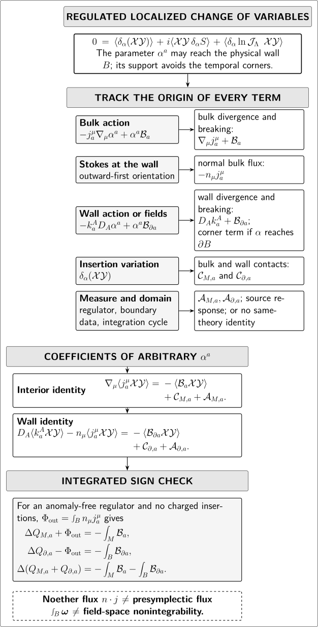
Every term has a distinct origin. Bulk and wall action variations supply divergences and explicit breaking, Stokes’ theorem supplies $-n_\mu j_a^\mu$, insertion variations supply contact distributions, and the regulated measure supplies $\mathcal A$. The integrated check defines positive $\Phi_{\mathrm{out}}$ to lower the bulk charge and raise an absorbing boundary charge. The final distinction prevents a spacetime current flux from being mistaken for presymplectic flux or field-space nonintegrability.

The diagram is equivalent to the following term-by-term account.

Origin	Term produced	When it may be absent
$-j_a^\mu\nabla_\mu\alpha^a$ in the bulk action	$\nabla_\mu j_a^\mu$ in the interior and $-n_\mu j_a^\mu$ on the wall	The normal term is hidden, not disproved, if $\alpha
$\alpha^a\mathcal B_a$ in the bulk action	Bulk explicit-breaking insertion	Exact regulated bulk symmetry
$-k_a^A D_A\alpha^a$ in the wall action	$D_Ak_a^A$ and, if the parameter reaches $\partial B$, a corner term	No boundary current; corner term also vanishes under the stated support choice
$\alpha^a\mathcal B_{\partial a}$ in the wall action	Boundary breaking or fixed-source response	Invariant fixed boundary data, or a covariant source family with its source variation retained
$\delta_\alpha\mathcal X$ and $\delta_\alpha\mathcal Y$	Bulk and wall contact distributions	Only when all insertions are invariant and no derivative contacts occur
$\delta_\alpha\ln\mathcal J_\Lambda$	Regulated bulk or boundary Jacobian contribution	Symmetry-preserving regulated measure
Variation of the integration domain or fixed boundary condition	A controlled source/domain response, or failure of the same-theory change-of-variables step	The transformation preserves the regulated domain and boundary problem

From local identities to charge balance

Remove charged insertions from the slab and assume an invariant regulated measure. Define

$$Q_{M,a}[\Sigma] =\int_\Sigma\mathrm d\Sigma_\mu\,j_a^\mu, \qquad \Phi_a[B_{12}] =\int_{B_{12}}\mathrm d\Sigma_\mu\,j_a^\mu,$$

where $\mathrm d\Sigma_\mu$ points outward on the wall. Stokes’ theorem gives

$$\begin{aligned} \int_{M_{12}}\!\mathrm d^d x\sqrt{-g}\, \nabla_\mu j_a^\mu ={}&Q_{M,a}[\Sigma_2]-Q_{M,a}[\Sigma_1] \\ &+\Phi_a[B_{12}]. \end{aligned}$$

Using $\nabla_\mu j_a^\mu=-\mathcal B_a$ therefore yields the bulk balance law

$$\begin{aligned} Q_{M,a}[\Sigma_2]-Q_{M,a}[\Sigma_1] +\Phi_a[B_{12}] =- \int_{M_{12}}\!\mathrm d^d x\sqrt{-g}\, \mathcal B_a. \end{aligned}$$

Positive outward flux contributes with the sign that lowers the later bulk charge. More generally, the bulk charge is cut independent exactly when $\Phi_a[B_{12}]+\int_{M_{12}}\sqrt{-g}\,\mathcal B_a=0$; nonzero terms can cancel. Separate vanishing is a simple sufficient condition. For an exact bulk symmetry, $\mathcal B_a=0$, zero net outward flux is necessary and sufficient. The local equation $\nabla_\mu j_a^\mu=0$ does not supply that flux condition.

If the wall has a charge

$$Q_{\partial,a}[S] =\int_S\mathrm dS_A\,k_a^A,$$

then the wall identity gives

$$\begin{aligned} Q_{\partial,a}[S_2]-Q_{\partial,a}[S_1] -\Phi_a[B_{12}] =- \int_{B_{12}}\!\mathrm d^{d-1}y\sqrt{|\gamma|}\, \mathcal B_{\partial a}. \end{aligned}$$

Adding the two equations cancels the exchange flux:

$$\begin{aligned} &\bigl(Q_{M,a}[\Sigma_2]+Q_{\partial,a}[S_2]\bigr) -\bigl(Q_{M,a}[\Sigma_1]+Q_{\partial,a}[S_1]\bigr) \\ &\quad=- \int_{M_{12}}\!\mathrm d^d x\sqrt{-g}\,\mathcal B_a - \int_{B_{12}}\!\mathrm d^{d-1}y\sqrt{|\gamma|}\, \mathcal B_{\partial a}. \end{aligned}$$

Thus an exact combined symmetry can conserve $Q_{M,a}+Q_{\partial,a}$ while neither summand is separately conserved. If there is no boundary current and no boundary breaking, the wall identity requires $n_\mu j_a^\mu=0$. If the wall is an external reservoir, the bulk charge can genuinely leak; the reservoir response then lies outside the closed bulk theory rather than disappearing from the balance law.

The displayed formulas exclude charged insertions and Jacobian terms only to make the transport statement transparent. Crossing a charged insertion adds its contact contribution. A nonzero $\mathcal A$ contributes its integrated bulk or boundary term with the sign fixed by its definition above.

Boundary conditions, equations, and sources

Three logically different ingredients are often described loosely as “the boundary condition.”

Ingredient	Logical role	Symmetry question
Imposed boundary condition	Restricts the histories and variations included in one theory, such as fixed Dirichlet or Robin data	Does the transformation map every admitted history and variation back into the same domain?
Boundary equation of motion	Follows by varying dynamical boundary values or boundary fields in a well-posed action	Does the equation implement exchange between bulk and boundary currents?
External boundary source	Labels a family of theories or generating functionals	Is the source transformed with the family, or held fixed as explicit breaking?

An invariant fixed boundary condition permits a change of variables inside the same path integral. A transforming source instead gives a covariant identity for a family of functionals. Holding a noninvariant source fixed removes its compensating variation and leaves $\mathcal B_{\partial a}$. If a formal transformation changes an imposed boundary condition and no controlled source or domain variation has been supplied, one cannot set the change of the original functional to zero.

A boundary equation of motion can numerically resemble Robin data, but its origin is different. It results from stationarity with respect to an admitted variation and can transfer charge to a dynamical wall field. An imposed Robin condition is part of the domain before the variation is performed. The variational distinction and the requirements for a well-posed action are developed in Boundaries, Variations, and Well-Posed Actions.

Complex scalar: reflection, injection, and exchange

Return to the charge-one complex scalar with

$$j^\mu =i\left( \phi^\dagger\partial^\mu\phi -(\partial^\mu\phi^\dagger)\phi \right), \qquad \delta\phi=i\phi.$$

Keep the controlled bulk deformation

$$\Delta\mathcal L =h\phi^N+h^*(\phi^\dagger)^N, \qquad N\geq2.$$

In the renormalized convention already established in the currents chapter,

$$[\mathcal B]_R =iN\left( h[\phi^N]_R -h^*[(\phi^\dagger)^N]_R \right).$$

Now add the real Robin coupling $\kappa$ and a charge-one external boundary source $f$:

$$S_B =\int_B\mathrm d^{d-1}y\sqrt{|\gamma|} \left( -\kappa\phi^\dagger\phi +f^\dagger\phi+\phi^\dagger f \right), \qquad \kappa\in\mathbb R.$$

Allowing the boundary value of $\phi$ to vary gives the natural equations

$$n_\mu\partial^\mu\phi-\kappa\phi+f=0, \qquad n_\mu\partial^\mu\phi^\dagger-\kappa\phi^\dagger+f^\dagger=0.$$

They imply

$$\begin{aligned} n_\mu j^\mu &=i\left[ \phi^\dagger(\kappa\phi-f) -(\kappa\phi^\dagger-f^\dagger)\phi \right] \\ &=i\left(f^\dagger\phi-\phi^\dagger f\right). \end{aligned}$$

This one calculation separates three cases.

• For $f=0$ and real $\kappa$, the Robin data are $U(1)$ invariant and $n_\mu j^\mu=0$: the wall is reflecting for this charge. Dirichlet and Neumann scalar walls are complementary finite-boundary examples in Harlow and Wu 2020, § 3.2, pp. 24–26, Open PDF.
• For fixed $f\neq0$, varying only $\phi$ gives $\mathcal B_\partial=i(f^\dagger\phi-\phi^\dagger f)$. Hence $-n_\mu j^\mu+\mathcal B_\partial=0$, exactly as required by the wall identity with $k^A=0$. The boundary source injects or removes bulk charge.
• If $f\mapsto e^{i\alpha}f$ is transformed together with $\phi\mapsto e^{i\alpha}\phi$, the boundary action is covariant. This is an identity for the source family, not a restoration of symmetry in one member with a fixed nonzero $f$.

To turn external injection into exchange with boundary matter, replace the source by a dynamical charge-one field $\chi$ and include, schematically,

$$\mathcal L_B =D_A\chi^\dagger D^A\chi-U(|\chi|^2) +\lambda\chi^\dagger\phi +\lambda^*\phi^\dagger\chi.$$

With

$$k^A =i\left( \chi^\dagger D^A\chi -(D^A\chi^\dagger)\chi \right),$$

the bulk and boundary equations give

$$D_Ak^A =i\left( \lambda\chi^\dagger\phi -\lambda^*\phi^\dagger\chi \right) =n_\mu j^\mu.$$

For $h=0$ and invariant boundary interactions, the same flux that lowers $Q_M$ raises $Q_\partial$, so the combined $U(1)$ charge is conserved. A fixed nonzero $h$ breaks the continuous $U(1)$ to $\mathbb Z_N$ only if the boundary data also preserve that subgroup. A generic fixed charge-one source $f$ breaks the residual subgroup as well. The finite $\mathbb Z_N$ identity has no nontrivial infinitesimal neighborhood and is not obtained by differentiating the current Ward identity.

Ordinary inflow, anomaly inflow, and other fluxes

Ordinary bulk-to-boundary inflow is the transport just derived: a propagating current has nonzero $n_\mu j^\mu$, and boundary matter or an external reservoir absorbs it. Anomaly inflow is different. There a regulated boundary Jacobian is canceled by the variation of an adjacent higher-dimensional effective action, so only the combined quantum system has an invariant generating functional. The cancellation must be checked in one regulator and counterterm scheme; it cannot be inferred from a classical normal current.

Perturbative boundary Ward identities and the higher-dimensional inflow picture are treated under explicit anomaly hypotheses in Thorngren and Wang 2021, § 2.1, pp. 4–7, and § 5, pp. 35–36, Open PDF. The general classification of regulated obstructions belongs to Anomalies, Inflow, and Matching.

Four nearby objects must remain distinct.

Object	Space on which it lives	Question it answers
$n_\mu j_a^\mu$	Spacetime wall	How much Noether charge crosses the wall?
$k_a^A$	Boundary spacetime	How do boundary degrees of freedom carry or transport that symmetry charge?
$\int_{B_{12}}\boldsymbol\omega(\delta_1,\delta_2)$	Spacetime boundary, valued in field-space two-forms	Does the presymplectic form change between hypersurfaces?
$\eta_\epsilon=\iota_{R_\epsilon}\Omega_\Sigma$	Field space	Is the candidate Hamiltonian one-form exact, so that a surface charge exists?

The first is the flux in this page’s balance law. The second is a boundary Ward current. The third is presymplectic flux. The fourth is the integrability question developed later. A nonzero Noether flux does not prove Hamiltonian nonintegrability, and an integrable charge need not be conserved. In the gravitational asymptotic setting, the structural separation between integrability and flux is explicit in Wald and Zoupas 2000, §§ 3–4, pp. 9–18, Open PDF; that application is not being generalized here without its hypotheses.

Common failure modes

Making the parameter vanish on the wall. This is a useful way to derive the interior identity, but it removes the terms needed to decide whether charge is reflected, exchanged, or leaked. It cannot establish a boundary Ward identity.

Promoting local conservation to charge conservation. Even when $\nabla_\mu j^\mu=0$, the bulk charge changes by minus the outward flux, so an exact bulk symmetry also needs zero net flux for cut independence. With explicit breaking, the exact condition is $\Phi+\int_M\sqrt{-g}\,\mathcal B=0$; a cancellation between the two terms is not separate conservation of either contribution.

Using a noninvariant boundary condition as a change of variables. If the transformation leaves the integration domain, it relates different boundary problems. Retain a controlled source/domain response or do not claim a same-theory identity.

Calling every boundary relation an equation of motion. Imposed boundary data restrict the domain; a boundary equation follows from an admitted variation. Only the latter automatically participates in a dynamical exchange equation.

Confusing $k_a^A$ with a surface-charge form. The former is a spacetime current tangent to the wall. The latter is a differential form on a codimension-two cut and is also linear in a field-space variation.

Calling a Jacobian term an anomaly immediately. A nontrivial regulated Jacobian is a candidate contribution. A genuine anomaly requires the renormalized identity, allowed counterterms, and consistency conditions.

Check your understanding

1. Recover the outward-flux sign

Starting from $\nabla_\mu j^\mu=-\mathcal B$, integrate over $M_{12}$ with the outward-first orientation. Show that positive wall flux lowers the later bulk charge.

Stokes’ theorem gives

$$\int_{M_{12}}\nabla_\mu j^\mu =Q_M[\Sigma_2]-Q_M[\Sigma_1]+\Phi[B_{12}].$$

Substitution of $\nabla_\mu j^\mu=-\mathcal B$ yields

$$Q_M[\Sigma_2]-Q_M[\Sigma_1] =-\Phi[B_{12}]-\int_{M_{12}}\mathcal B.$$

For an exact bulk symmetry, $\mathcal B=0$, so $\Phi>0$ implies $Q_M[\Sigma_2]<Q_M[\Sigma_1]$.

2. Distinguish a fixed source from a covariant source family

For the scalar boundary coupling $f^\dagger\phi+\phi^\dagger f$, compare varying only $\phi$ with varying $f$ as a charge-one source.

If $f$ is held fixed,

$$\delta_\alpha S_B =\int_B\alpha\, i(f^\dagger\phi-\phi^\dagger f),$$

so $\mathcal B_\partial=i(f^\dagger\phi-\phi^\dagger f)$. If $\delta f=i\alpha f$ is included, the source variation cancels this term. The second statement relates functionals at transformed source values; it does not make a single fixed nonzero-$f$ theory $U(1)$ invariant.

3. Check conservation with dynamical boundary matter

Assume $\mathcal B=\mathcal B_\partial=0$ and $D_Ak^A=n_\mu j^\mu$. Integrate the bulk and boundary equations and show that only the total charge is forced to be constant.

The bulk equation gives $\Delta Q_M=-\Phi$, while the boundary equation gives $\Delta Q_\partial=+\Phi$. Therefore

$$\Delta(Q_M+Q_\partial)=0.$$

Neither $Q_M$ nor $Q_\partial$ is separately constant unless the exchange flux vanishes.

4. Test the residual finite symmetry

With fixed nonzero $h$, which phase rotations survive $h\phi^N+h^*(\phi^\dagger)^N$? What happens if a generic fixed charge-one boundary source is also present?

The bulk deformation is invariant when $e^{iN\alpha}=1$, leaving $\mathbb Z_N$. A generic fixed $f$ requires $e^{i\alpha}=1$ for the linear boundary coupling to be invariant, so it removes every nontrivial element of that residual subgroup. Because $\mathbb Z_N$ is finite, this conclusion is a finite transformation statement, not an infinitesimal current identity.

What to carry forward

A localized symmetry variation that reaches a boundary produces two coupled Ward identities. The interior equation contains bulk divergence, explicit breaking, contacts, and any bulk Jacobian. The wall equation balances normal bulk flux against a tangential boundary current, boundary breaking or source response, boundary contacts, and any boundary Jacobian. Their integrated form states exactly when a bulk charge leaks, when a boundary charge absorbs the flux, and when a total charge is conserved.

For a gauge transformation, continue next to Proper and Improper Gauge Transformations to determine whether the allowed transformation is a null redundancy or a physical boundary symmetry. Only after that classification should a proposed Hamiltonian charge be tested on Surface Charges, Integrability, and Ambiguities. For limiting falloffs and scattering interfaces, use Asymptotic Symmetry, Soft Limits, and the Boundary Interface. Physical boundary interactions and defect operator data continue on Boundaries, Interfaces, and Domain Walls.

References

• Billò, Marco, Vasco Gonçalves, Edoardo Lauria, and Marco Meineri. “Defects in Conformal Field Theory.” Journal of High Energy Physics 2016, no. 4 (2016): 091. DOI. Open PDF
• Harlow, Daniel, and Jie-Qiang Wu. “Covariant Phase Space with Boundaries.” Journal of High Energy Physics 2020, no. 10 (2020): 146. DOI. Open PDF
• Schwartz, Matthew D. Quantum Field Theory and the Standard Model. Cambridge: Cambridge University Press, 2014. DOI
• Thorngren, Ryan, and Yifan Wang. “Anomalous Symmetries End at the Boundary.” Journal of High Energy Physics 2021, no. 9 (2021): 017. DOI. Open PDF
• Wald, Robert M., and Andreas Zoupas. “A General Definition of ‘Conserved Quantities’ in General Relativity and Other Theories of Gravity.” Physical Review D 61, no. 8 (2000): 084027. DOI. Open PDF