Gauge Structure, Global Form, and Observables

Use this chapter when a local gauge potential is no longer enough to specify the physical question. An ordinary compact gauge theory in the settings considered here is assembled in layers: local connections and matter fields, admissible bundle sectors and boundary data, the subgroup whose orbits are treated as redundancy, observables or dressed charged insertions, and the global gauge group and its representations. In the four-dimensional line-spectrum branch, genuine-line and discrete-theta data add another layer; disconnected transformations require their own classical and quantum decisions. Changing one layer can change the theory even when every local formula in a chosen gauge looks the same.

The chapter follows two intersecting progressions. The first runs from admissible transformations through Gauss law and the redundancy quotient to invariant or dressed observables. The second runs from local potentials through bundles and sectors to global form, genuine lines, topological weights, and disconnected transformations. Boundary conditions and the actual global group connect the two: they determine which transformations are available, which have zero generators, which representations exist, and constrain which extended probes can be defined.

The seven topic pages form two main routes rather than one compulsory course. Choose the route matching the object you need to classify. The chapter stops before detailed boundary-charge algebras, gauge-fixed quantization, renormalized defect construction, anomaly tests, and model-dependent gauge dynamics.

Helpful background. The Free Maxwell Field and Gauge Redundancy supplies the controlled spin-one model, while Bundle Connections, Curvature, Gauge Transformations, and Bianchi Identities supplies the geometric connection language. Neither is a hard prerequisite for using this overview.

Parent volume. Symmetry and Gauge Structure

Jump to: choose a route · review the chapter

Diagnose your preparation

Use the observable checks below rather than a score. An Unsure result means that the Repair link is the efficient starting point; it does not bar entry to this overview.

Free Maxwell theory. Ready: You can identify the Gauss constraint, the two propagating polarizations, and gauge-invariant field strengths; enter Gauge Fields. Unsure: You know $A_\mu\mapsto A_\mu+\partial_\mu\lambda$ but cannot say what is constrained or observable. Repair: Use The Free Maxwell Field and Gauge Redundancy and, before the orbit route, Maxwell Constraints as a Worked Application.

Connections. Ready: You can distinguish a connection from its local potential and state that non-Abelian curvature transforms covariantly; enter Gauge Fields. Unsure: You can manipulate $A_\mu$ but do not know how it changes under a local frame change. Repair: Use Bundle Connections, Curvature, Gauge Transformations, and Bianchi Identities.

Bundles and patches. Ready: You can explain why local potentials on overlaps require transition functions; enter Global Configurations. Unsure: You expect every smooth field strength to come from one global potential. Repair: Use Vector, Principal, and Associated Bundles.

Constrained reduction. Ready: You can separate a constraint surface, its null directions, and the quotient by those directions; enter Gauge Orbits. Unsure: You treat imposing Gauss law and choosing a gauge condition as the same operation. Repair: Use Constraints, Dirac Brackets, and Symplectic Reduction.

Representation descent. Ready: You can compute a representation kernel and test whether an action descends through a quotient; enter Global Form. Unsure: You identify Lie-algebra representations with representations of every global form. Repair: Use Representations, Intertwiners, Invariants, and Tensor Decomposition.

Homotopy and degree. Ready: You can interpret a based map’s winding as a homotopy class; enter Large Transformations after the global-configuration page. Unsure: You identify a bundle’s characteristic number with a component of its automorphism group. Repair: Use Homotopy, Degree, Winding, and Covering Spaces.

Choose by the question you need to answer

Reader goal	Route	Capability at the end
Build the subject from a first gauge-field example	Gauge Fields $\to$ Orbits $\to$ Global Configurations $\to$ Dressed Observables	Separate representatives, the Gauss-law quotient, bundle sectors, and observable completions
Decide whether a transformation is redundant or physically charged	Gauge Fields $\to$ Orbits $\to$ Dressed Observables $\to$ Proper and Improper Gauge Transformations	Test the complete differentiable generator instead of classifying a transformation from its local formula or boundary value alone
Specify a gauge theory beyond its Lie algebra	Gauge Fields $\to$ Global Configurations $\to$ Global Form $\to$ Genuine Lines $\to$ Large Transformations	State the bundle, group, representation, line-spectrum, topological-weight, and transformation-component data that the problem actually uses
Construct or classify an observable	Gauge Fields $\to$ Orbits $\to$ Dressed Observables $\to$ Wilson Lines and Loops	Distinguish a local singlet, a completed open transporter, a boundary-dressed charge, and a renormalized line-operator problem
Compare $\operatorname{SU}(2)$ , $\operatorname{SO}(3)_+$ , and $\operatorname{SO}(3)_-$	Global Configurations $\to$ Global Form $\to$ Genuine Lines	Separate bundle and representation data from the additional choice of a mutually local genuine-line spectrum
Track topology or theta phases	Global Configurations $\to$ Global Form $\to$ Genuine Lines $\to$ Large Transformations $\to$ Theta Terms, Periodicity, and Vacuum Sectors	Keep field sectors, discrete-theta data, transformation components, consistent quantum characters, and topological actions distinct

Arrows in the table mean suggested reading order, not logical implication. The sidebar is reference order, not prerequisite order. The reduction-and-observable branch is pages 1 $\to$ 2 $\to$ 4. The global specification branch is pages 1 $\to$ 3 $\to$ 5 $\to$ 6, while page 7 can be entered from page 3 after the homotopy preparation above. These focused routes assume the hard inputs named in the diagnostic: Maxwell constraints and symplectic reduction before page 2, representation theory before page 5, and homotopy degree before page 7.

Two progressions meet in the physical quotient

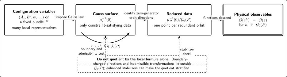
Fix a spatial region, boundary or falloff data, an actual gauge group, and a set $\mathfrak S$ of allowed principal-bundle classes. For a representative $P$ of each class, let $\mu_P=0$ denote the Gauss-constraint surface. Let $\mathcal G_0(P)$ denote the full subgroup actually declared redundant. Its identity-connected directions are generated by complete differentiable generators with zero differential on the allowed constraint surface, after normalizing any fixed constant. Any disconnected components included in $\mathcal G_0(P)$ are additional global input; Gauss law does not generate them. With that declaration made, the reduced phase space has the schematic form

\mathcal P_{\mathrm{phys}} \simeq \coprod_{[P]\in\mathfrak S} \frac{\mu_P^{-1}(0)}{\mathcal G_0(P)}.

The bundle-sector sum is developed on Local Potentials and Global Gauge Configurations; the constraint surface and regular reduction are developed on Gauge Orbits, Gauss Constraints, and Stabilizers; and the boundary-sensitive choice of $\mathcal G_0$ begins on Gauge Fields, Redundancy, and Observable Content.

This display is an organizing map, not a theorem covering every singular or quantum case. Enhanced stabilizers can make the coarse quotient stratified, and a quantum state can be a section of a nontrivial line bundle over the classical quotient rather than an ordinary function on it, as developed for the bounded based-action example on Large Gauge Transformations and Topological Sectors. The constraint-to-orbit relation is developed in Tong 2018, § 2.2.1, pp. 40–42, official PDF; orbit-type stratification is treated in Vilela Mendes 2004, §§ 2 and 3.1, pp. 2–4 and 6–8, Open PDF.

The reduction map below makes the order of operations visible. Within one fixed bundle sector, first impose Gauss law, then identify only the orbit directions generated by the subgroup actually declared redundant. Gauge-invariant observables are precisely the functions that descend through that quotient.

Configuration variables are restricted to the Gauss surface, quotiented only along zero-generator gauge orbits, and then mapped to invariant observables — Classical gauge reduction in one fixed bundle sector, shown schematically and not to scale. Gauss law restricts the configuration data; quotienting by $\mathcal G_0(P)$ identifies zero-generator orbit directions; physical observables are constant on those orbits. Boundary-charged or inadmissible transformations are not included merely because they share the same local gauge formula, and enhanced stabilizers can make the quotient stratified.

An observable on this reduced space must be constant along the $\mathcal G_0(P)$ orbits. A charged insertion can instead be equivariant under a physical boundary or global symmetry after its redundant variation has been removed by endpoints, a dressing, or relational data. Which transformations belong to $\mathcal G_0(P)$ cannot be read from whether their parameters vanish at a boundary. For identity-connected transformations, the action, allowed variations, and complete generator decide whether the direction is redundant or physically charged. For disconnected components, membership in the redundancy subgroup or retention as a physical action is a separate global declaration. A possible quantum character is then an additional question, not a third mutually exclusive classical role. The boundary-sensitive quotient and charge distinction is developed in Harlow and Wu 2020, § 1, pp. 3–4, and § 3.3, pp. 22–23, Open PDF.

The second progression asks what must be declared before that schematic quotient names one theory. Local potentials $A_i$ and transition functions $h_{ij}$ specify a connection on a bundle $P$ . The Lie algebra fixes the infinitesimal connection law, but for a compact connected semisimple algebra the connected global forms are central quotients. For a representation $\rho:\widetilde G\to\operatorname{GL}(V)$ ,

\begin{gathered} G_\Gamma=\widetilde G/\Gamma, \\ \rho\text{ descends to }G_\Gamma \\ \Longleftrightarrow\Gamma\subseteq\ker\rho. \end{gathered}

Even the global group and matter representations need not complete a four-dimensional gauge theory: a complete mutually local spectrum of genuine line charges and compatible discrete-theta data can distinguish theories with the same $G_\Gamma$ . The basic $\operatorname{SO}(3)_+$ and $\operatorname{SO}(3)_-$ comparison is explained in Aharony, Seiberg, and Tachikawa 2013, §§ 1–1.3, pp. 1–6, Open PDF and placed in the generalized-symmetry framework in Bhardwaj et al. 2024, §§ 3.3.3–3.4, pp. 46–49 and 53–57, Open PDF.

The following nonvisual map keeps the layers separate:

Question	Governing object	What it does not decide by itself
Which local representative is being used?	Potentials $A_i$ and local frame choices	The bundle class or physical quotient
Which field sector is allowed?	Bundle class $[P]\in\mathfrak S$ and transition data	Which automorphisms are redundant
Which infinitesimal directions are removed?	Gauss law and the identity-connected zero-generator directions in $\mathcal G_0(P)$	Which disconnected components are also declared redundant
Why can orbit dimension jump?	The stabilizer of a representative	A universal smooth coordinate system on the full quotient
Which quantities are physical?	Functions invariant under $\mathcal G_0(P)$ , or charged objects with explicit completion data	Locality, finiteness, or renormalization
Which matter and Wilson representations exist?	The global group and representation-descent condition	The complete genuine-line spectrum
Which electric, magnetic, or dyonic lines are genuine?	A complete mutually local reduced charge subgroup $L$	Screening, confinement, or long-distance phase behavior
Which transformations are large?	Components $\pi_0(\mathcal G_{\mathcal B}(P))$ of the admissible group	Whether a component is included in the redundancy quotient or retained as a physical action
How can declared redundant components act on quantum states?	Equivariance under the residual component group; in the bounded based-action example, a character or flat-line-bundle holonomy	Whether the component was large or whether a different component carries a physical charge

Read the rows from top to bottom for global specification. Read the third, fourth, and fifth rows together for reduction to observables. The bundle and boundary rows connect the two readings.

Exact chapter guide

1. Gauge Fields, Redundancy, and Observable Content

Start here to determine what an ordinary Lie gauge field is, which admissible transformations are redundant, and which combinations can represent observable content. It fixes the local connection law, the boundary-sensitive definition of $\mathcal G_0$ , and the first Maxwell comparison among orbit, charge, and gauge-fixed descriptions. After this page, you can separate a local representative from orbit and observable data. It requires the free Maxwell field and bundle connections. Continue to the orbit page for systematic reduction, the global-configuration page for patching, or the dressing page for observable construction.

2. Gauge Orbits, Gauss Constraints, and Stabilizers

This page supplies the systematic reduction. It asks how the Gauss constraint generates null orbit directions and why enhanced stabilizers obstruct one regular quotient chart. It derives the regular polarization count and uses an $\operatorname{SU}(2)$ holonomy model to expose orbit-type jumps. After this page, you can recognize when the regular quotient picture fails because the stabilizer changes. It requires the first page, constrained symplectic reduction, and the worked Maxwell constraints. Continue to global configurations, dressed observables, or the later boundary-charge chapter.

3. Local Potentials and Global Gauge Configurations

This page supplies the global field description. It asks how local potentials and transition functions define one global connection and how bundle topology labels distinct field sectors. Its compact $U(1)$ example shows why local field equations do not select the sector sum. After this page, you can distinguish a bundle sector from a gauge orbit inside that sector. It requires the first page and principal-bundle patching. Continue to global form when the group and representations matter, or to large transformations when bundle automorphisms and their components are the target.

4. Gauge-Invariant and Dressed Observables

Use this page to construct observables. It asks how a covariant field or open transporter can be completed into an object invariant under $\mathcal G_0$ . It distinguishes local singlets, neutral bilocals, boundary-dressed charges, and the Gauss-law obstruction to compactly localized charge-changing operators. After this page, you can identify what completion data a proposed charged observable is missing. It requires the orbit page; parallel transport is helpful. Continue to global form for allowed endpoint representations, to extended operators for renormalized lines, or to scattering for infrared dressings.

5. Global Form, Matter Representations, and the Faithful Gauge Group

This page tests global-form descent. It asks how covers, central quotients, and representation kernels determine the connected group acting faithfully on specified matter. It separates the Lie algebra, the chosen global group, and the faithful matter quotient without claiming that matter reconstructs the full theory. After this page, you can test whether matter or a Wilson representation descends to a chosen global form. It requires global-configuration data and representation theory. Continue to the line-spectrum page for the additional theory data invisible to local matter.

6. Genuine Line Spectra, Discrete Theta Data, and Theory Specification

This page completes the four-dimensional line-spectrum data. It asks why the Lie algebra and connected global group can still leave distinct four-dimensional theories. It develops the reduced mutual-locality test and distinguishes $\operatorname{SU}(2)$ , $\operatorname{SO}(3)_+$ , and $\operatorname{SO}(3)_-$ through their genuine electric, magnetic, and dyonic lines. After this page, you can explain why $\operatorname{SO}(3)_+$ and $\operatorname{SO}(3)_-$ are distinct despite sharing a Lie algebra and global group. It requires the global-form page. Continue to large transformations for component phases or to extended operators for construction, screening, and fusion.

7. Large Gauge Transformations and Topological Sectors

This page separates topology, the classical quotient, and the quantum character. It asks when an admissible transformation is disconnected, whether its component is included in the redundancy quotient or retained as a physical action, and independently how quantum states may transform by a theta character. It separates transformation components from bundle sectors and works through based $\operatorname{SU}(2)$ transformations on a three-ball. After this page, you can make the classical quotient and quantum-character decisions separately. It requires global configurations and homotopy degree; global form is helpful. Continue to topological terms, instanton dynamics, global anomalies, or theorem-level bundle automorphisms according to which additional question remains.

Conventions that carry across the chapter

The site-wide conventions apply. The formulas throughout this chapter use Hermitian Lie-algebra generators and $D_\mu=\partial_\mu-igA_\mu$ ; the four-dimensional examples use the mostly-minus metric $(+---)$ and the quantum action phase $e^{iS}$ . Local gauge laws, curvature, transporters, and topological phases must be translated as a complete set when a source uses anti-Hermitian generators or the opposite sign in $D_\mu$ .

Several notation distinctions are more important than any sign:

$\mathcal G_{\mathcal B}(P)$ is the group of transformations admissible for the chosen bundle and boundary data. $\mathcal G_0(P)$ is the full subgroup declared redundant: its identity-connected directions pass the zero-generator test, while any disconnected components included in it are separate global input. It need not equal $\mathcal G_{\mathcal B}(P)^\circ$ .
$\mathfrak g$ , $\widetilde G$ , a quotient $G_\Gamma$ , and the group acting faithfully on a specified matter spectrum answer different questions.
A non-Abelian curvature is covariant; traces and other invariant contractions produce gauge-invariant local quantities.
A genuine line needs no attached topological surface. The word does not mean unscreened, topological, deconfined, or finite after renormalization.
A large transformation is disconnected in the stated admissible group. Disconnectedness alone determines neither its classical role nor the character by which a redundant component may act on quantum states.
Theta periodicity and discrete-theta formulas depend on the global group, allowed manifolds, and boundary completion. The chapter never assumes one universal period.

The central-quotient statement used here is scoped to compact connected semisimple groups. Abelian factors and disconnected gauge groups require additional global data.

Two bounded-region threads expose the layers

The chapter uses two controlled threads. Each keeps some data fixed and changes others deliberately, so a conceptual difference is not hidden by a wholesale change of model.

Maxwell and compact U(1): redundancy to charged observables

The fixed starting point is an Abelian gauge field in $3+1$ dimensions on a region with boundary. Pages 1 and 2 distinguish Gauss-law orbit directions from finite, integrable boundary generators and recover the two regular bulk polarizations. Page 3 then declares the global group compact and uses a spherical shell: patch data permit quantized magnetic flux although the local Maxwell equations do not choose a sector sum. Page 4 returns to matter and shows that a charge-changing completion must reach another charge, the boundary, or infinity.

Compactness and the shell topology are controlled changes; the local Abelian connection law stays fixed. The recurrent check is always the same: Which data are local, which label a sector, and which transformation has a nonzero generator? The thread stops before edge-mode dynamics, renormalized Wilson lines, monopole cores, one-form-symmetry breaking, and compact-BF response. Those questions continue in the boundary, extended-operator, higher-form, topological-term, and nonperturbative chapters.

The su(2) thread: local algebra to global theory

Here the fixed data are four spacetime dimensions and the local $\mathfrak{su}(2)$ Yang–Mills connection law. Page 3 supplies the bundle language. Page 5 changes the connected global form from $\operatorname{SU}(2)$ to $\operatorname{SO}(3)$ and tracks the resulting bundle and Wilson-representation differences. Page 6 holds the $\operatorname{SO}(3)$ group fixed but changes the genuine magnetic or dyonic line spectrum, distinguishing $\operatorname{SO}(3)_+$ from $\operatorname{SO}(3)_-$ . Page 7 changes both the global group back to $\operatorname{SU}(2)$ and the bounded spatial geometry to a three-ball, in order to isolate the component group of based $\operatorname{SU}(2)$ transformations and the independent theta-character choice.

The recurrent check is whether a proposed distinction belongs to the Lie algebra, global group, bundle sector, line spectrum, transformation component, or quantum character. The thread does not compute confinement, instanton weights, or phase dynamics. As in the Abelian thread, a closed-manifold topological phase cannot be copied onto a bounded spacetime without boundary data or a relative gluing prescription.

The operator-centered continuation begins on Gauge-Invariant and Dressed Observables: Wilson and dressed objects lead through global form and the reduced charge lattice here, then to Genuine Lines, Screening, and Charge Lattices, Linking, Braiding, and Framing, and Fusion, Junctions, and Endpoints. Electric and Magnetic One-Form Symmetries then interprets the resulting operator data as generalized symmetry before higher-form gauging and higher-group mixing. This chapter stops at theory specification; it does not construct those renormalized defects or their fusion rules.

What local formulas cannot decide

The chapter’s strongest synthesis is a chain of counterexamples:

The same Lie algebra need not define the same global group.
The same global group need not define the same genuine-line theory.
The same local gauge transformation can be redundant under one set of boundary conditions and physically charged under another.
A disconnected component may be included in the classical redundancy quotient while states carry a consistent character, or it may be retained as a physical action. Topology alone decides neither the classical role nor the quantum phase.
A gauge-fixed local action can hide every preceding distinction without erasing it.

Accordingly, a complete problem statement for the theories treated here should answer, in order: What is the local field and matter content? Which bundles and boundary data are allowed? Which identity-connected directions have zero generators, and which disconnected components are separately declared redundant? What stabilizers occur? Which observables or dressings descend to the quotient? What is the global group and which representations descend? In the four-dimensional line-spectrum branch, which genuine lines and topological weights are part of the theory? Finally, how do disconnected components act on quantum states? If one applicable answer is missing, the apparent calculation may be comparing representatives, sectors, or theories without saying so.

This decision sequence does not replace the later dynamics. It specifies the kinematic and global data on which confinement, Higgs behavior, instantons, renormalization, anomalies, and scattering dressings depend.

Boundaries and canonical exits

For differentiable generators, surface charges, and edge-mode choices, continue to Boundary Symmetry, Surface Charges, and Edge Modes.
For Faddeev–Popov determinants, ghosts, BRST cohomology, BV fields, and Gribov limitations, continue to Gauge Fixing, BRST, and BV.
For inconsistent global phases rather than consistent theta characters, continue to Anomalies, Inflow, and Matching.
For renormalized lines, screening, junctions, and defects, continue to Extended Operators and Defects.
For one-form symmetry generated by topological operators, continue to Higher-Form and Higher-Group Symmetries.
For topological actions and their boundary completion, continue to Topological Terms and Invertible Responses.
For interacting model dynamics and matter content, use Dynamical Gauge Fields and Matter.
For monopoles, instantons, confinement, and theta-state dynamics, use Nonperturbative Dynamics; for asymptotic charged dressings, use Dressed States and Infrared-Finite Scattering.
For theorem-first orbit spaces, bundle automorphisms, or charged sectors, continue to Mathematical Gauge Theory or Gauss-Law Charges and Infrared Sectors.

Review the chapter

Each prompt names the expected work product, a success criterion, and the first repair route.

Use this repair map: local representatives and redundancy belong to Gauge Fields and Gauge Orbits; bundles belong to Global Configurations; dressings belong to Gauge-Invariant and Dressed Observables; global-group descent belongs to Global Form; genuine lines belong to Genuine Lines; and disconnected components belong to Large Transformations.

Retrieval and explanation — classify the data. For one bounded gauge theory, list a local potential, curvature, bundle class, admissible transformation group, identity-connected zero-generator subgroup, any separately declared disconnected redundancies, stabilizer, invariant local observable, dressed charged object, global group, and genuine-line datum. Use the conceptual map and the repair map above. A successful response gives each item a different role and does not call $A_\mu$ or non-Abelian $F_{\mu\nu}$ an invariant observable. Repair at the first unmatched category in the linked map.

Derivation — trace the Maxwell reduction. Starting from canonical Maxwell data, show how Gauss law and one redundant orbit direction remove one canonical pair, then state the boundary-flux condition needed before the generator is set to zero. Use pages 1 and 2. Success means obtaining two configuration-space polarizations while keeping the boundary generator test separate from the local constraint. Repair on Gauge Orbits, Gauss Constraints, and Stabilizers.

Convention translation — compare two gauge laws. Translate a source that uses anti-Hermitian generators or $D_\mu=\partial_\mu+igA_\mu$ into the chapter’s Hermitian-generator convention. Use pages 1 and 3. Success means that the transformed covariant derivative, curvature, transporter endpoints, and overlap laws remain mutually consistent; changing the sign of $A$ in one formula only is a failure. Repair on Bundle Connections, Curvature, Gauge Transformations, and Bianchi Identities.

Comparison and failure diagnosis — separate three theories. Compare $\operatorname{SU}(2)$ , $\operatorname{SO}(3)_+$ , and $\operatorname{SO}(3)_-$ at fixed Lie algebra. Use pages 3, 5, and 6. A successful response distinguishes allowed representations and bundles from the magnetic or dyonic genuine-line choice, and explains why a local Faddeev–Popov operator cannot recover the missing data. Repair on Global Form, Matter Representations, and the Faithful Gauge Group before returning to the line-spectrum page.

Transfer — change the boundary conditions. Take a Maxwell or Yang–Mills transformation whose parameter is allowed to be nonzero at the boundary. State what must be recomputed before calling it redundant, charged, or inadmissible. Use pages 1, 2, 4, and 7. Success means naming preservation of the field space, differentiability, the surface variation, integrability, and the action on observables. For a disconnected component, it must also separate the declared classical role from any quantum character; the boundary value or connected component alone is not an answer. Repair on Gauge Fields, Redundancy, and Observable Content and then continue to Proper and Improper Gauge Transformations.

Synthesis — complete an underspecified theory. Given only a local $\mathfrak g$ -valued Lagrangian, write the shortest list of additional data needed before its sectors, physical quotient, charged observables, and line operators are determined. Use all seven pages. Success is a typed sequence covering bundles and boundaries, identity-connected zero-generator reduction, any declared disconnected redundancies, stabilizers, global form and matter descent, applicable genuine-line and topological data, and the independent quantum action of disconnected components. Use the corresponding linked page in the repair map to repair the first omitted layer.

Continue from here

For the shortest structural route, read Gauge Fields, Redundancy, and Observable Content, Gauge Orbits, Gauss Constraints, and Stabilizers, and Local Potentials and Global Gauge Configurations. Add Gauge-Invariant and Dressed Observables when the target is an operator, or continue through global form, genuine lines, and large transformations when the target is complete theory specification.

The most common next step is Proper and Improper Gauge Transformations for boundary charges, The Faddeev–Popov Construction for local quantization, or Genuine Lines, Screening, and Charge Lattices for extended probes.

Return to the Symmetry and Gauge Structure overview to choose another chapter or compare this route with the volume’s current, boundary, anomaly, and generalized-symmetry branches.

References

Aharony, Ofer, Nathan Seiberg, and Yuji Tachikawa. “Reading between the Lines of Four-Dimensional Gauge Theories.” Journal of High Energy Physics 08 (2013): 115. DOI. Open PDF
Bhardwaj, Lakshya, Lea E. Bottini, Ludovic Fraser-Taliente, Liam Gladden, Dewi S. W. Gould, Arthur Platschorre, and Hannah Tillim. “Lectures on Generalized Symmetries.” Physics Reports 1051 (2024): 1–87. DOI. Open PDF
Harlow, Daniel, and Jie-qiang Wu. “Covariant Phase Space with Boundaries.” Journal of High Energy Physics 10 (2020): 146. DOI. Open PDF
Tong, David. Gauge Theory. Cambridge Part III Mathematical Tripos lecture notes, University of Cambridge, 2018. Official course page. Official PDF
Vilela Mendes, R. “Stratification of the Orbit Space in Gauge Theories: The Role of Nongeneric Strata.” Journal of Physics A: Mathematical and General 37, no. 47 (2004): 11485–11498. DOI. Open PDF