Scalar Propagators, Ordered Correlators, and Sources

For a free massive real scalar in the selected Minkowski vacuum, one normalized mode expansion fixes the two Wightman distributions. The commutator, retarded and advanced Green kernels, and time- and anti-time-ordered correlators are then obtained by adding different algebraic, support, ordering, and boundary data. They are not interchangeable: even when their momentum-space expressions contain the same off-shell factor $p^2-m^2$, they have different distributional meanings and satisfy different Klein–Gordon equations.

This page works in $d$-dimensional Minkowski spacetime with $m>0$ and the vacuum representation constructed in the preceding page. All point-field formulas denote distributions and acquire their operator meaning after smearing. Thermal and curved-spacetime states, interacting or gauge-field propagators, Euclidean continuation, and the massless infrared limit are outside the present scope.

Required background. Quantizing the Real Scalar Field supplies the normalized mode expansion, oscillator algebra, selected Minkowski vacuum, and equal-time commutator used below.

Helpful background. Holomorphic Functions and Cauchy Theory and Laurent Series, Poles, and Residues supply the energy-contour calculation. Tempered Distributions and Fourier Calculus supplies on-shell delta distributions and boundary values. Fundamental Solutions and Green Operators and Hyperbolic Equations and Causal Propagators supply the inverse and support conditions used to identify the retarded and advanced kernels.

Vacuum Wightman functions from the scalar mode expansion

Write $z=x-y$, set $P=\Box+m^2$, and retain the invariant on-shell measure from the quantized scalar:

$$\begin{aligned} \int_{\mathbf p} &\equiv \int \frac{\mathrm d^{d-1}\mathbf p} {(2\pi)^{d-1}2E_{\mathbf p}}, \\ E_{\mathbf p} &=\sqrt{\mathbf p^2+m^2}. \end{aligned}$$

Contracting the mode expansion against the selected vacuum leaves one annihilator–creator term:

$$\begin{aligned} W^+(z) &\equiv \langle0|\widehat\phi(x)\widehat\phi(y)|0\rangle \\ &= \int_{\mathbf p}e^{-ip\cdot z}, \\ W^-(z) &\equiv \langle0|\widehat\phi(y)\widehat\phi(x)|0\rangle \\ &=W^+(-z) = \int_{\mathbf p}e^{+ip\cdot z}. \end{aligned}$$

Here $p^0=E_{\mathbf p}$ in the on-shell integrals. Equivalently, with the site Fourier convention understood,

$$\begin{aligned} \widetilde W^+(p) &= 2\pi\,\theta(p^0)\delta(p^2-m^2), \\ \widetilde W^-(p) &= 2\pi\,\theta(-p^0)\delta(p^2-m^2). \end{aligned}$$

Thus

$$PW^+=PW^-=0.$$

The two distributions are homogeneous bisolutions, not inverses of $P$. Their positive- or negative-energy support records the chosen vacuum, and neither is confined to a position-space causal cone. In particular, $W^+(0,\mathbf r)$ is generally nonzero for $\mathbf r\neq0$: spacelike vacuum correlation is not the same thing as causal response. The contraction, time-ordering decomposition, and its normalization are derived in Schwartz 2014, § 6.2, pp. 75–77; the convention-translated structural treatment is in Weinberg 1995, § 6.2, pp. 274–277.

The commutator and causal inverses

For the linear free field, the operator commutator is a c-number distribution times the identity. Define that distribution by

$$\begin{aligned} [\widehat\phi(x),\widehat\phi(y)] &= C(z)\mathbf1, \\ C(z) &= W^+(z)-W^-(z). \end{aligned}$$

Its momentum-space form is

$$\begin{aligned} \widetilde C(p) &= 2\pi\,\operatorname{sgn}(p^0) \delta(p^2-m^2), \\ PC&=0. \end{aligned}$$

The normalization can be checked without any contour argument. At equal time,

$$\begin{aligned} C(0,\mathbf r)&=0, \\ \left. \partial_{z^0}C(z^0,\mathbf r) \right|_{z^0=0} &= -i\delta^{(d-1)}(\mathbf r). \end{aligned}$$

Since $\partial_{y^0}=-\partial_{z^0}$, this gives

$$[\widehat\phi(t,\mathbf x), \widehat\pi(t,\mathbf y)] = i\delta^{(d-1)}(\mathbf x-\mathbf y)\mathbf1,$$

so the two-point normalization returns exactly to the canonical algebra. Lorentz invariance gives a second check: every spacelike $z$ can be transformed to an equal-time separation, where $C$ vanishes. Hence $C$ has causal support even though $W^\pm$ do not.

Two neighboring pages use different standard names for this same distributional data. If

$$[\widehat\phi(x),\widehat\phi(y)] =i\Delta(z)\mathbf1$$

and the Mathematical Methods causal propagator is

$$E=G_{\mathrm{ret}}-G_{\mathrm{adv}},$$

then the accepted crosswalk is

$$\begin{aligned} C&=i\Delta=-iE, \\ E&=iC, \\ \Delta&=-E. \end{aligned}$$

This sign is fixed by the equal-time derivative, not by notation. The delta-normalized support-selected inverses are therefore

$$\begin{aligned} G_{\mathrm{ret}}(z) &= i\theta(z^0)C(z), \\ G_{\mathrm{adv}}(z) &= -i\theta(-z^0)C(z). \end{aligned}$$

Using $C(0,\mathbf r)=0$ and its derivative jump gives

$$\begin{aligned} P G_{\mathrm{ret}} &=\delta^{(d)}, & \operatorname{supp}G_{\mathrm{ret}} &\subseteq J^+(0), \\ P G_{\mathrm{adv}} &=\delta^{(d)}, & \operatorname{supp}G_{\mathrm{adv}} &\subseteq J^-(0). \end{aligned}$$

Their full momentum boundary values are

$$\begin{aligned} \widetilde G_{\mathrm{ret}}(p) &= -\frac{1} {(p^0+i0)^2-E_{\mathbf p}^2}, \\ \widetilde G_{\mathrm{adv}}(p) &= -\frac{1} {(p^0-i0)^2-E_{\mathbf p}^2}. \end{aligned}$$

Both retarded poles lie below the real $p^0$ axis, whereas both advanced poles lie above it. Their difference is the homogeneous causal propagator $E=iC$; it is not itself an inverse. The separation between a state-independent free-field commutator and state-dependent two-point functions is developed in Hollands and Wald 2015, § 2.1, pp. 9–14, Open PDF. State independence here belongs to the linear free-field algebra, not to arbitrary interacting composite operators.

Time ordering and the Feynman boundary value

The vacuum time-ordered correlator is

$$\begin{aligned} D_F(z) &\equiv \langle0|\mathrm T \widehat\phi(x)\widehat\phi(y)|0\rangle \\ &= \theta(z^0)W^+(z) +\theta(-z^0)W^-(z). \end{aligned}$$

For each spatial momentum, the required energy integral is

$$\begin{aligned} I_F(t,\mathbf p) &= \int\frac{\mathrm dp^0}{2\pi} \frac{i\,e^{-ip^0t}} {(p^0)^2-E_{\mathbf p}^2+i0} \\ &= \frac{1}{2E_{\mathbf p}} \left[ \begin{aligned} &\theta(t)e^{-iE_{\mathbf p}t} \\ &+\theta(-t)e^{+iE_{\mathbf p}t} \end{aligned} \right]. \end{aligned}$$

For $t>0$ the contour closes below and encloses the positive-energy pole; for $t<0$ it closes above and encloses the negative-energy pole. Restoring the spatial transform gives

$$D_F(z) = \int\frac{\mathrm d^d p}{(2\pi)^d} \frac{i\,e^{-ip\cdot z}} {p^2-m^2+i0}.$$

Thus the positive-energy pole lies below and the negative-energy pole above the real axis. Applying $P$ either to the momentum boundary value or to the step-function form yields the contact term

$$P D_F=-i\delta^{(d)}.$$

The anti-time-ordered companion reverses both the ordering and the pole displacement:

$$\begin{aligned} D_{\bar F}(z) &\equiv \langle0|\overline{\mathrm T} \widehat\phi(x)\widehat\phi(y)|0\rangle \\ &= \theta(-z^0)W^+(z) +\theta(z^0)W^-(z), \\ \widetilde D_{\bar F}(p) &= -\frac{i}{p^2-m^2-i0}, \\ P D_{\bar F} &= +i\delta^{(d)}. \end{aligned}$$

Two quick algebraic checks are

$$\begin{aligned} D_F+D_{\bar F} &=W^++W^-, \\ D_F-D_{\bar F} &=\operatorname{sgn}(z^0)C. \end{aligned}$$

The raw vacuum correlator $D_F$ is not the delta-normalized mathematical inverse. With the Green-operator convention used above,

$$G_F=iD_F, \qquad P G_F=\delta^{(d)}.$$

Forgetting this factor of $i$ is enough to reverse the source normalization. The contour derivation and the independent contact-term calculation agree with Schwartz 2014, § 6.2, pp. 75–77 and, after translating both signature and correlator prefactors, Weinberg 1995, § 6.2, pp. 274–277.

Sources select different boundary data

There are two distinct source questions. First add a classical c-number source with the site sign convention,

$$S_J=S_0+\int\mathrm d^d x\,J(x)\phi(x).$$

The sourced equation is $P\phi_J=J$. If the sourced part has no incoming field, its solution is

$$\phi_J = \phi_{\mathrm{hom}} +G_{\mathrm{ret}}*J.$$

The support condition, not the differential equation alone, selects $G_{\mathrm{ret}}$. Choosing final rather than initial support would select $G_{\mathrm{adv}}$.

The normalized vacuum source amplitude asks another question. Define the source-dependent ordered exponential and its vacuum amplitude by

$$\begin{aligned} \mathcal U_J &\equiv \mathrm T\exp\!\left( i\int\mathrm d^d x\,J\widehat\phi \right), \\ Z_0[J] &\equiv \langle0|\mathcal U_J|0\rangle, \\ Z_0[0]&=1. \end{aligned}$$

Differentiating the definition twice gives

$$\begin{aligned} \left. \frac{\delta^2Z_0[J]} {\delta J(x)\delta J(y)} \right|_{J=0} &= i^2D_F(x-y), \\ D_F(x-y) &= \left. \frac{1}{i^2} \frac{\delta^2Z_0[J]} {\delta J(x)\delta J(y)} \right|_{J=0}. \end{aligned}$$

The vacuum and the time-ordering symbol are already part of $Z_0$, so ordinary derivatives generate the Feynman correlator—not the retarded response. To first order about the same vacuum, define the real-time response kernel

$$\begin{aligned} \chi(x,y) &\equiv \left. \frac{\delta\langle\widehat\phi(x)\rangle_J} {\delta J(y)} \right|_{J=0}, \\ \chi(x,y) &= i\theta(x^0-y^0)C(x-y) \\ &= G_{\mathrm{ret}}(x-y). \end{aligned}$$

The two derivatives differ because their state-contour and support questions differ. The exact free Gaussian functional and the full hierarchy of normalized and connected source derivatives belong to Gaussian Fields and Sources and The Generating Functional. The plus-sign source convention and Feynman boundary condition are developed in Schwartz 2014, §§ 14.3–14.4, pp. 261–266.

One family, different defining data

The dependency map should be read from top to bottom. A solid arrow takes the free-field difference, a double arrow imposes operator ordering in the selected vacuum, and a dashed arrow imposes future or past support. Inspect the pole arrows only for the four off-shell boundary values; the Wightman functions and commutator instead live on the mass shell.

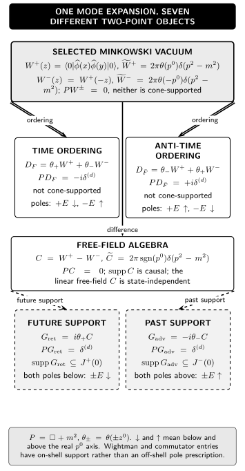
One normalized free-scalar mode expansion supplies $W^+$ and $W^-$ in the selected Minkowski vacuum, but difference, ordering, and support operations define different two-point objects. $C$, $W^+$, and $W^-$ are homogeneous bisolutions; $D_F$ and $D_{\bar F}$ have opposite contact terms and pole placements; $G_{\mathrm{ret}}$ and $G_{\mathrm{adv}}$ are delta-normalized inverses with future and past support. Arrows below or above the real $p^0$ axis encode pole placement, not position-space support. The diagram is schematic for the massive linear free field.

The semantic tables below spell out every leaf of the map without relying on its geometry or line styles. The main distinctions can therefore be read without relying on the overloaded word “propagator.”

Object	Mathematical type and defining data	Klein–Gordon equation
$W^+$	vacuum correlator in the written operator order	$PW^+=0$
$W^-$	vacuum correlator in the reverse operator order	$PW^-=0$
$C$	free-field commutator fixed by the algebra	$PC=0$
$G_{\mathrm{ret}}$	inverse selected by future support	$PG_{\mathrm{ret}}=\delta^{(d)}$
$G_{\mathrm{adv}}$	inverse selected by past support	$PG_{\mathrm{adv}}=\delta^{(d)}$
$D_F$	vacuum time-ordered correlator	$PD_F=-i\delta^{(d)}$
$D_{\bar F}$	vacuum anti-time-ordered correlator	$PD_{\bar F}=+i\delta^{(d)}$

Object	Position-space support	Momentum-space selection
$W^+$	not cone-supported	positive-energy mass shell
$W^-$	not cone-supported	negative-energy mass shell
$C$	causal cone	signed mass shell
$G_{\mathrm{ret}}$	future cone	both energy poles below
$G_{\mathrm{adv}}$	past cone	both energy poles above
$D_F$	not cone-supported	positive-energy pole below, negative-energy pole above
$D_{\bar F}$	not cone-supported	positive-energy pole above, negative-energy pole below

Momentum-space mass-shell support and position-space causal support are different statements. Likewise, the bare expression $1/(p^2-m^2)$ does not define a distribution across the mass shell. For one real variable,

$$\frac{1}{u\pm i0} = \operatorname{PV}\frac1u \mp i\pi\delta(u),$$

so changing the boundary value changes the on-shell term even though the functions agree away from $u=0$. A principal-value kernel, a Feynman boundary value, and a retarded boundary value are therefore different distributions. The denominator identifies the differential operator; the state, ordering, support, and boundary prescription identify the two-point object.

Uses, limits, and continuations

This construction is exact for the continuum linear free field in the selected massive Minkowski vacuum. $W^\pm$ and the ordered correlators change when the state changes, while the c-number commutator and its retarded and advanced kernels remain fixed by the same free-field algebra. In an interacting theory the field commutator is generally operator-valued, and its expectation value need not be state-independent. A finite momentum cutoff can also spoil exact spacelike cancellation, so continuum microcausality should not be inferred from a truncated mode sum without a regulator analysis.

The next developed questions are separated by purpose:

• Fock Space, Vacuum, and Particle Number develops the representation generated by the selected vacuum and the representation dependence of particle number.
• Gaussian Fields and Sources derives the regulated Gaussian source functional, while the Canonical–Functional Crosswalk compares it with this canonical result under matched regulators.
• Lorentzian Boundary Conditions and the iε Prescription develops convergence factors, vacuum boundary data, and contour deformations beyond the one-energy integral used here.
• Massless Scalars, Zero Modes, and Infrared Limits treats $m\to0$, finite volume, dimension dependence, and the zero mode.
• The Fermion Propagator adds the Dirac numerator, spin sums, and fermionic ordering signs.

Common pitfalls

Calling a Wightman function an inverse. $W^\pm$ solve the homogeneous equation and encode state data. They do not produce a delta source under $P$.

Calling the Feynman correlator causal response. The Feynman $i0$ prescription implements vacuum time ordering, not future-cone support. Its nonzero spacelike correlations do not permit signaling; retarded response is selected by $G_{\mathrm{ret}}$.

Dropping the correlator prefactor. $D_F$ obeys $PD_F=-i\delta^{(d)}$, whereas the mathematical inverse is $G_F=iD_F$. Mixing them changes source equations and every subsequent source derivative.

Generalizing the free commutator too far. State independence follows here because the linear free-field commutator is a c-number fixed by the canonical algebra. It is not a statement about arbitrary interacting fields or composite operators.

Check your understanding

1. Retrieval. Define $W^+$, $W^-$, $C$, and $D_F$. Which of them require the selected vacuum, and which require an ordering prescription?
2. Distinction. Two momentum expressions reduce to $1/(p^2-m^2)$ away from the mass shell. What additional data are needed before they can be identified as distributions?
3. Normalization and contour. Derive $\partial_{z^0}C(0,\mathbf r)=-i\delta^{(d-1)}(\mathbf r)$ and $PD_F=-i\delta^{(d)}$. Place the two energy poles for the Feynman, anti-time-ordered, retarded, and advanced prescriptions.
4. Failure mode. Diagnose the claims “$W^+$ is a Green inverse,” “Feynman means future-causal,” and “$D_F$ is the delta-normalized inverse.”
5. Transfer. A compact classical source is switched on with no incoming sourced field. Separately, a vacuum source amplitude is differentiated twice. Which kernel answers each question, and why are they different?
6. Handoff. Where should you continue for the full Gaussian source calculation, a sustained $i0$ analysis, the massless limit, or the fermion numerator?

Answers and repair routes

1. $W^+(z)=\langle0|\widehat\phi(x)\widehat\phi(y)|0\rangle$, $W^-(z)=W^+(-z)$, $C=W^+-W^-$, and $D_F=\theta(z^0)W^++\theta(-z^0)W^-$. $W^\pm$ and $D_F$ require the selected vacuum; $D_F$ additionally requires time ordering. The free commutator $C$ is fixed by the algebra. Repair the starting normalization at Quantizing the Real Scalar Field.
2. One must specify the boundary value at the mass shell, pole placement or on-shell delta contribution, defining equation and normalization, position-space support, operator ordering, and state data where applicable. Review tempered Fourier calculus for boundary values and causal propagators for support-selected inverses.
3. Differentiating $W^+-W^-$ at $z^0=0$ cancels the $2E_{\mathbf p}$ in the measure and leaves $-i$ times the spatial Fourier representation of the delta. Differentiating the step functions in $D_F$ then produces $PD_F=-i\delta^{(d)}$. Feynman places $+E_{\mathbf p}$ below and $-E_{\mathbf p}$ above; anti-time ordering reverses them; retarded places both below; advanced places both above. Repair the residue step at Laurent series, poles, and residues.
4. The first claim fails because $PW^+=0$, not $\delta$. The second confuses frequency boundary data with cone support: $D_F$ is not future-supported. The third misses the raw-correlator factor, since $PD_F=-i\delta$ and $G_F=iD_F$ is the delta-normalized inverse.
5. The no-incoming classical response is $G_{\mathrm{ret}}*J$ because future support is part of the problem. Two ordinary derivatives of the normalized time-ordered vacuum amplitude give $D_F$ because the vacuum and $\mathrm T$ are built into its definition. A shared differential operator does not erase those different selection data.
6. Use Gaussian Fields and Sources for the regulated Gaussian derivation, Lorentzian Boundary Conditions and the iε Prescription for the full boundary-value analysis, Massless Scalars, Zero Modes, and Infrared Limits for $m\to0$, and The Fermion Propagator for spinor numerators and fermionic ordering.

References

• Hollands, Stefan, and Robert M. Wald. “Quantum Fields in Curved Spacetime.” Physics Reports 574 (2015): 1–35. DOI. Open PDF.
• Schwartz, Matthew D. Quantum Field Theory and the Standard Model. Cambridge: Cambridge University Press, 2014. DOI.
• Weinberg, Steven. The Quantum Theory of Fields, Volume I: Foundations. Cambridge: Cambridge University Press, 1995. First edition; 2005 paperback, 2012 printing consulted. DOI.

References

Section titled “References”- Hollands, Stefan, and Robert M. Wald. “Quantum Fields in Curved Spacetime.” Physics Reports 574 (2015): 1–35. DOI. Open PDF: 2014 arXiv v2 preprint; locators above use its printed page labels.