States, Observables, and Spectra

A quantum field is useful because its matrix elements probe states, not because every field component is directly observable. In a vacuum two-point function, inserting a complete set of energy–momentum states turns those matrix elements into a spectral measure. The measure then separates isolated stable-particle weight from multiparticle continua, and the Källén–Lehmann transform turns that separation into a precise distinction among poles, thresholds, and cuts.

This chapter follows the chain

$$\text{matrix elements} \longrightarrow \text{spectral measure} \longrightarrow \text{Källén–Lehmann form} \longrightarrow \text{analytic structure},$$

then asks where particle language succeeds or fails. A stable isolated mass shell, a resonance pole reached by analytic continuation, and an infraparticle threshold are three different structures. Only the first can enter the ordinary scattering route, and even then a pole is not by itself an LSZ theorem.

Choose an entry route · Read the spectral map · Review the chapter

Enter this chapter

Let $|\Omega\rangle$ be a translation-invariant vacuum and let $\mathcal O$ be a Hermitian scalar operator in a positive-metric physical Hilbert space. Subtract its vacuum expectation,

$$\widehat{\mathcal O} =\mathcal O -\langle\Omega|\mathcal O|\Omega\rangle\mathbf 1,$$

so the vacuum itself does not appear as a zero-momentum contribution. Translation covariance and a complete set of physical energy–momentum states resolve the Wightman function

$$W_{\mathcal O}(x) =\langle\Omega| \widehat{\mathcal O}(x)\widehat{\mathcal O}(0) |\Omega\rangle$$

into positive squared overlaps. With the spectrum in the closed forward cone and scalar Poincaré covariance, those overlaps assemble into a nonnegative measure $\rho_{\mathcal O}(\mu^2)\,\mathrm d\mu^2$. Whenever the time-ordered extension requires no additional local terms, its scalar Källén–Lehmann form is

$$\widetilde D_{F,\mathcal O}(p) = \int_0^\infty \mathrm d\mu^2\, \rho_{\mathcal O}(\mu^2) \frac{i}{p^2-\mu^2+i0}, \qquad \rho_{\mathcal O}\ge 0.$$

The positivity statement uses the physical positive inner product and Hermiticity; translation covariance fixes the momentum phases; the spectrum condition fixes support; and scalar covariance reduces the measure to invariant mass. The completeness derivation and positive scalar measure are developed in Schwartz 2014, § 24.2.1, pp. 467–469. Distributional regularity is also required. Locality is not used in this basic two-point completeness argument, although it becomes essential in stronger QFT and scattering results. General composite time-ordered products can require subtractions or local contact terms; in that case the displayed equality is understood modulo those local terms, while the Wightman spectral measure remains the clean primary statement.

If $\widehat{\mathcal O}$ has nonzero overlap with a stable scalar state of mass $m$ and that state is isolated from the continuum in the same quantum-number channel, then, in the simplest one-particle-plus-continuum case,

$$\begin{aligned} \rho_{\mathcal O}(\mu^2) &=Z_{\mathcal O}\,\delta(\mu^2-m^2) +\rho_{\mathrm{cont}}(\mu^2), \\ Z_{\mathcal O}&>0, \qquad \operatorname{supp}\rho_{\mathrm{cont}} \subseteq [s_0,\infty), \qquad s_0>m^2, \end{aligned}$$

where $s_0$ is the lightest allowed multiparticle invariant mass in that channel. It need not be $4m^2$. The transform becomes

$$\widetilde D_{F,\mathcal O}(p) =\frac{iZ_{\mathcal O}}{p^2-m^2+i0} +i\int_{s_0}^{\infty}\mathrm d\mu^2\, \frac{\rho_{\mathrm{cont}}(\mu^2)} {p^2-\mu^2+i0}.$$

The delta atom produces an isolated physical-sheet pole; continuous support produces a threshold branch point and cut in the infinite-volume limit. These structures may coexist. The residue $Z_{\mathcal O}$ depends on how $\mathcal O$ is normalized: rescaling the operator rescales both $Z_{\mathcal O}$ and $\rho_{\mathcal O}$. Therefore neither $\int\rho_{\mathcal O}=1$ nor $Z_{\mathcal O}\le1$ is asserted for an arbitrary operator. Schwartz 2014, § 24.2.1, p. 469; § 24.3, pp. 471–474 gives the pole-plus-continuum argument, while Weinberg 1995, § 10.2, pp. 430–434 explains why the pole criterion depends on a nonzero matrix element rather than on whether a field is called elementary or composite.

The chapter stops at three boundaries. It identifies a resonance with a complex pole on an analytically continued, channel-dependent nonphysical sheet—not with a normalizable unstable ket or merely a bump. It introduces an infraparticle as a long-range infrared case in which continuous spectral weight reaches the nominal mass and the isolated mass-shell atom can disappear—not as a resonance with a width. Finally, it states the stable-pole, overlap, asymptotic-state, separation, and infrared conditions that permit a scattering handoff, but it does not derive LSZ reduction. Detailed sheet analysis, infrared constructions, and scattering amplitudes continue in later volumes.

Check your preparation

The overview imposes no prerequisite; each leaf states its own required and helpful background. Use the repair links below when a step is not yet routine.

Try this	Ready when	Repair if unsure
Compare a field, an observable, and an interpolating operator	You can explain why a field may have useful matrix elements without itself being a directly measurable observable	Quantum states and operators repair, then Fields, Observables, and Interpolating Operators
Insert a complete set between two operators	You can identify which assumptions turn the terms into nonnegative squared overlaps and which operator quantum numbers restrict the intermediate states	Vacua, States, and Representations
Normalize a one-particle state covariantly	You can use $\langle\mathbf p’	\mathbf p\rangle=2E_{\mathbf p}(2\pi)^3\delta^{(3)}(\mathbf p’-\mathbf p)$ without losing a phase-space factor
Compare Wightman and time-ordered two-point functions	You can identify the ordering, vacuum, Fourier convention, and $+i0$ prescription before interpreting a denominator	The Generating Functional and Scalar Propagators, Ordered Correlators, and Sources
Read a positive spectral measure and a resolvent boundary value	You can distinguish a point mass from continuous support and a physical boundary value from analytic continuation to another sheet	Spectra, Resolvents, Spectral Measures, and Functional Calculus and Branches, Sheets, Analytic Continuation, and Monodromy

Choose a route

The six leaves have a coherent reading order, but the chapter has three useful entrances. “Required” below names an actual dependency; other sequencing is a recommendation chosen for the stated goal.

Reader goal	Route through the chapter	Observable exit
Understand what operator data mean	Operators, Observables, and Matrix Elements → Spectral Decomposition of Two-Point Functions → The Källén–Lehmann Representation. The first page requires the earlier states and interpolating-operator pages; the second additionally requires the generating functional.	Insert completeness, derive the scalar spectral support, and state exactly why the measure is nonnegative
Translate spectral support into analytic structure	Spectral Decomposition → Källén–Lehmann → Poles, Cuts, Thresholds, and Stable Particles. Helpful mathematics comes from spectral measures, branches, and dispersion integrals.	Map a delta atom to a stable pole and continuum support to a threshold cut without calling the cut a particle
Test particle language and scattering readiness	Poles, Cuts, Thresholds, and Stable Particles → Resonances, Infraparticles, and Limits of Particle Language for the contrast. For the ordinary scattering route, combine the poles-and-cuts page with Fields, Observables, and Interpolating Operators, then read From One-Particle Poles to the Scattering Handoff.	Decide whether the data support an ordinary stable external state, a resonance analysis, an infrared-modified framework, or no particle claim at all

The spectral content map

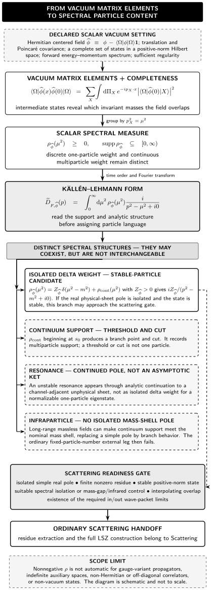
Read the upper path in the figure from matrix elements to the Källén–Lehmann transform. Then compare the spectral components below it. An isolated delta atom and continuum support can occur together; the later resonance and infraparticle labels require additional analytic or infrared information and do not follow from the mere existence of a continuum.

Schematic spectral-content map for a vacuum-subtracted Hermitian scalar operator in a positive-metric physical Hilbert space. The stable delta atom and continuum may coexist. Resonance and infraparticle branches are conditional diagnoses, while the ordinary scattering handoff additionally requires an isolated shell, nonzero overlap, suitable in/out limits, and infrared control; the diagram is not a quantitative spectrum and is not to scale.

The same relationships can be read without the image.

Input or feature	Licensed conclusion	What does not follow
Vacuum matrix elements, completeness, translation covariance, the forward spectrum, scalar covariance, and a positive physical inner product	A nonnegative invariant-mass measure for a Hermitian scalar operator	Locality, clustering, a mass gap, or asymptotic completeness
Källén–Lehmann transform of that measure	A time-ordered two-point function built from free-mass denominators with the common $+i0$ boundary value	Positivity for gauge-variant components in an indefinite auxiliary space or for arbitrary off-diagonal and non-vacuum correlators
Isolated $Z_{\mathcal O}\delta(\mu^2-m^2)$	A simple physical-sheet pole with nonnegative operator-dependent residue and a stable one-particle contribution	That the state is elementary, that $Z_{\mathcal O}\le1$, or that LSZ assumptions are already satisfied
Continuous support from $s_0$	A threshold branch point and cut in the infinite-volume limit	A new particle at the threshold, or automatically a resonance or infraparticle
Pole reached by continuation through a channel cut	A resonance diagnosis with explicit sheet and channel conventions	A normalizable unstable one-particle ket or an ordinary LSZ external state
Continuous threshold behavior at a nominal charged mass because arbitrarily soft quanta cannot be separated	Possible infraparticle behavior with no isolated mass-shell pole	A decay width, a resonance interpretation, or one universal threshold exponent
Stable isolated shell, finite nonzero overlap, suitable asymptotic limits and separation, plus infrared and physical-state control	Readiness to begin the ordinary scalar scattering reduction	The LSZ derivation itself or asymptotic completeness of the whole theory

The six pages in order

The guide below lists every leaf once in its dependency order.

1. Operators, Observables, and Matrix Elements. Required background is Vacua, States, and Representations together with Fields, Observables, and Interpolating Operators. Distinguish an operator from a measurement prescription, identify the state dependence of matrix elements, and explain how an interpolating operator can reveal a particle sector without being an observable in every sense.

2. Spectral Decomposition of Two-Point Functions. Required background is the first page and The Generating Functional. Helpful background comes from Bounded, Compact, and Integral Operators and Spectra, Resolvents, Spectral Measures, and Functional Calculus. Insert completeness, use translation covariance, and derive the positive scalar spectral sum or measure before introducing the propagator representation.

3. The Källén–Lehmann Representation. Required background is the spectral-decomposition page; spectra and resolvents are helpful. Derive the scalar representation with its minimal vacuum, covariance, spectrum, completeness, positivity, and regularity assumptions visible. Identify which steps do not use locality and where composite, gauge-fixed, or non-vacuum cases require new qualifications.

4. Poles, Cuts, Thresholds, and Stable Particles. Required background is Källén–Lehmann. Helpful background comes from Spectra, Resolvents, Spectral Measures, and Functional Calculus, Branches, Sheets, Analytic Continuation, and Monodromy, and Boundary Values, Discontinuities, and Dispersion Integrals. Translate discrete and continuous spectral support into the physical-sheet pole, threshold, and cut dictionary, including the finite-volume qualification.

5. Resonances, Infraparticles, and Limits of Particle Language. Required background is the poles-and-cuts page. Contrast an analytically continued resonance pole with an infrared threshold lacking an isolated mass shell. This page supplies the conceptual warning; detailed resonance extraction continues in Scattering, and developed infraparticle theory continues in Scattering, Gauge Theories, and Mathematical QFT.

6. From One-Particle Poles to the Scattering Handoff. Required background is the poles-and-cuts page together with Fields, Observables, and Interpolating Operators. State the pole, residue, normalization, asymptotic-state, isolation, and infrared hypotheses needed before ordinary scattering reduction can begin. Resonances and infraparticles are failure or modification cases, but page 5 is not a hard prerequisite for this stable-particle route.

Conventions that control the spectrum

The chapter inherits the site’s $(+---)$ metric. The following page-local data prevent the same spectral symbol from silently changing meaning.

Datum	Chapter convention	Check before reuse
Vacuum subtraction	$\widehat{\mathcal O}=\mathcal O-\langle\Omega	\mathcal O
State normalization	$\langle\mathbf p’	\mathbf p\rangle=2E_{\mathbf p}(2\pi)^3\delta^{(3)}(\mathbf p’-\mathbf p)$
Fourier transform	$f(p)=\int\mathrm d^4x\,e^{ip\cdot x}f(x)$, with inverse phase $e^{-ip\cdot x}$	A source using the opposite phase has all momentum labels translated consistently
Ordering and state	$D_{F,\mathcal O}=\langle\Omega	T\widehat{\mathcal O}\widehat{\mathcal O}
Spectral variable	The measure is written $\rho_{\mathcal O}(\mu^2)\,\mathrm d\mu^2$ on $\mu^2\ge0$	Factors associated with a density in $\mu$ rather than $\mu^2$ are not dropped
Positivity	$\rho_{\mathcal O}\ge0$ for a Hermitian scalar operator in the declared positive physical space	Gauge-variant, ghost, non-Hermitian, off-diagonal, and non-vacuum cases are separately qualified
Boundary value	Every scalar denominator is $i/(p^2-\mu^2+i0)$	A physical boundary value is distinguished from continuation through a cut
Residue symbol	$Z_{\mathcal O}$ is the operator’s one-particle overlap weight	It is not the source functional $Z[J]$ and is not normalization-independent
Sheet language	“Physical sheet” refers to the boundary value fixed by $+i0$; another sheet is reached by a declared analytic continuation	A resonance pole is never drawn or described as a first-sheet stable pole

The free scalar as a baseline

For the canonically normalized free real scalar, take $\mathcal O=\phi$ and $\langle\Omega|\phi|\Omega\rangle=0$. Completeness has one one-particle contribution in the field’s channel and no interacting multiparticle continuum, so

$$\rho_0(\mu^2)=\delta(\mu^2-m^2), \qquad \widetilde D_F^{(0)}(p) =\frac{i}{p^2-m^2+i0}.$$

This is the round-trip check for every later convention: the spectral integral must reproduce the same Feynman function obtained canonically and from the generating functional. If the field is rescaled, $\phi\mapsto c\phi$, the density becomes $c^2\delta(\mu^2-m^2)$; positivity survives, but the normalization changes.

An interacting operator can retain an isolated atom while acquiring continuum weight,

$$\delta(\mu^2-m^2) \quad\longrightarrow\quad Z_{\mathcal O}\delta(\mu^2-m^2) +\rho_{\mathrm{cont}}(\mu^2).$$

That single change supplies the chapter’s recurring comparison. The atom gives the stable pole. The continuum gives the threshold cut. A resonance requires analytic continuation beyond that physical boundary, and an infraparticle instead removes the isolated sharp-mass contribution through long-range infrared structure. None of those last three statements is obtained by renaming the free pole.

What the six pages say together

Question	Strongest conclusion in this chapter	Category error prevented
What physical information does a field carry?	Its state-dependent matrix elements can probe sectors with matching quantum numbers	Every field component is an observable
Why is the scalar spectral measure positive?	Its weights are squared overlaps in a positive physical Hilbert space for a Hermitian scalar operator	Every propagator or spectral matrix is entrywise positive
What does an isolated spectral atom mean?	It gives a stable one-particle contribution and a physical-sheet pole when the mass shell is isolated	Every pole is a particle, regardless of sheet or state status
What does a continuum mean?	In infinite volume it produces threshold support and a cut	Every threshold or cut is a particle
What distinguishes a resonance?	A channel- and sheet-qualified pole appears after analytic continuation; no normalizable unstable one-particle ket is implied	A line-shape bump is automatically a state or a resonance pole
What distinguishes an infraparticle?	Long-range soft structure can replace the isolated mass shell by continuous threshold behavior	An infraparticle is merely a resonance with a small width
When may ordinary scattering reduction begin?	Only after stable-pole, overlap, asymptotic-state, isolation, wave-packet, infrared, and physical-state conditions are stated	The handoff is already the LSZ derivation or a proof of asymptotic completeness

For resonances, the relevant distinction between physical and unphysical sheets—and the warning that a bump is neither necessary nor sufficient—is summarized in Particle Data Group 2025, “Resonances,” § 50.1.1, pp. 3–6 (PDF). For the infrared contrast, Buchholz 1986, pp. 331–334 proves, under its Gauss-law hypotheses, that charged states cannot be mass-operator eigenstates. The chapter uses that result as a bounded example, not as a universal claim about every massless theory.

Review the chapter

Use the stated criteria to identify exactly which physical or analytic step needs revision, then follow the corresponding repair route.

Check	A successful response must show	Repair route
Operator classification	Give one field that serves as an interpolating operator, state which matrix element matters, and explain why this alone does not define a measurement	Fields, Observables, and Interpolating Operators
Positivity derivation	Insert completeness into $W_{\mathcal O}(x)$ and point to the exact use of Hermiticity, the positive inner product, translation covariance, and the spectrum condition	Spectral Decomposition of Two-Point Functions
Free normalization	Substitute $\rho_0(\mu^2)=\delta(\mu^2-m^2)$ into the Källén–Lehmann integral and recover $i/(p^2-m^2+i0)$	The Källén–Lehmann Representation
Singularity classification	Given an isolated delta plus continuum from $s_0$, identify the pole and cut, and explain why the threshold itself is not a particle	Poles, Cuts, Thresholds, and Stable Particles
Failure diagnosis	Contrast a second-sheet resonance pole with continuous spectral behavior beginning at a nominal charged mass; state why neither is an ordinary stable external ket	Resonances, Infraparticles, and Limits of Particle Language
Scattering readiness	List the data missing from the statement “the two-point function has a pole” before an ordinary LSZ calculation may begin	From One-Particle Poles to the Scattering Handoff
Computational design	For a supplied discrete-plus-continuum measure, specify a quadrature, convergence test, error estimate, and the continuum claim that finite data would not establish	Spectral Decomposition of Two-Point Functions

Where to go next

• Return to the volume map: Foundations of Quantum Field Theory places this spectral chapter among states, quantization, sources, local operators, and spacetime formulations.

• Strengthen the mathematics: Mathematical Methods leads to spectral measures, resolvents, analytic continuation, and dispersion integrals without replacing the physical-state hypotheses used here.

• Design a reconstruction: Spectral Decomposition of Two-Point Functions supplies the analytic measure-to-correlator map. A runnable companion would additionally need declared inputs, quadrature, convergence tests, and an error budget; none is assumed here.

• Develop resonance or stable-particle scattering: Resonance Poles, Riemann Sheets, and Unstable States treats the continued-sheet analysis, while LSZ Reduction: Poles, Residues, and Stable External States supplies the full stable-state reduction.

• Develop infrared particle concepts: Infraparticles and Velocity Superselection gives the theorem-oriented route.

• Repair quantum-state language: Quantum states and operators repair revisits states, operators, representations, and observables.

• Track the open infrared problem: Infrared-Complete Scattering Observables collects the Research route rather than turning a live question into a settled foundation claim.

References

• Buchholz, Detlev. “Gauss’ Law and the Infraparticle Problem.” Physics Letters B 174 (1986): 331–334. DOI.

• Particle Data Group. “Resonances.” In Review of Particle Physics, 2025 update. Official PDF.

• Schwartz, Matthew D. Quantum Field Theory and the Standard Model. Cambridge: Cambridge University Press, 2014. DOI.

• Weinberg, Steven. The Quantum Theory of Fields, Volume I: Foundations. Cambridge: Cambridge University Press, 1995. DOI.