Fields, Configurations, Dimensions, and Local Dynamics

A classical local field model specifies a spacetime, admissible field configurations with their transformation and reality properties, a local density built from the fields and finitely many derivatives, parameters and scales, and an allowed class of boundary or initial data. The field type and configuration space are kinematic choices; the action supplies the dynamical law; particular boundary or initial data pose a problem whose solutions can then be sought.

This page develops that distinction for free scalar, Dirac, Proca, and Maxwell fields in four-dimensional Minkowski spacetime. It also derives their engineering dimensions. It does not yet vary the action, solve the field equations, analyze Hamiltonian constraints, count physical polarizations, or classify couplings by renormalization-group behavior.

Helpful background. Vector Spaces, Duals, Linear Maps, and Bases helps distinguish a field from its chosen components. Direct Sums, Tensor Products, and Index Structure helps interpret Lorentz, spinor, and internal indices.

The data of a classical local field model

Let $M$ be Minkowski spacetime. After choosing the standard flat-space trivializations used on this page, all four examples can be represented componentwise as maps

$$\Phi:M\longrightarrow V, \qquad x\longmapsto\Phi^A(x),$$

where $V$ is the appropriate component space and $A$ collectively labels field species and components. This local notation is sufficient for the present comparison; global bundle and connection data are developed in Mathematical Methods rather than here.

An off-shell raw configuration is an entire admissible field $\Phi$ in a space $\mathcal F_{\mathrm{raw}}$. Its definition includes kinematic requirements such as regularity, reality, and transformation law. A field value $\Phi^A(x)$ is only the value of one configuration at one point. An on-shell configuration additionally satisfies the dynamical equations $\mathcal E(\Phi)=0$, but need not satisfy a particular choice of initial or boundary data. If $D$ denotes those selected data, the solutions of the posed problem form

$$\operatorname{Sol}(D) = \left\{ \Phi\in\mathcal F_{\mathrm{raw}} \mathrel{\big|} \mathcal E(\Phi)=0 \quad\text{and}\quad \Phi\text{ satisfies }D \right\}.$$

In a gauge theory, an admissible gauge group $\mathcal G_{\mathrm{adm}}$ acts on raw configurations while preserving the declared regularity and problem data. Its subgroup $\mathcal G_{\mathrm{red}}\subseteq\mathcal G_{\mathrm{adm}}$ consists of transformations treated as descriptive redundancies. Where the quotient is well behaved, a physical solution is an orbit in $\operatorname{Sol}(D)/\mathcal G_{\mathrm{red}}$, not a preferred representative. Transformations in $\mathcal G_{\mathrm{adm}}\setminus\mathcal G_{\mathrm{red}}$ can instead act as physical symmetries and carry boundary charges; transformations that fail to preserve the declared data are not in $\mathcal G_{\mathrm{adm}}$ at all. Thus a point value, a raw configuration, an on-shell configuration, a solution of a posed problem, and a physical gauge orbit are distinct notions.

The separation among field space, solution space, gauge reduction, and boundary-sensitive symmetries is developed in Harlow and Wu 2020, § 1, pp. 3–4; §§ 2.1–2.2, pp. 5–12; § 3.3, pp. 22–23. This page uses only that structural distinction, not their full covariant phase-space construction.

For a local model of finite derivative order $r$, the action on a region $\Omega\subset M$ has the schematic form

$$S_\Omega[\Phi] = \int_\Omega \mathrm d^d x\, \mathcal L\!\left( x,\Phi,\partial\Phi,\ldots,\partial^{(r)}\Phi; g_I \right),$$

where $g_I$ denotes masses, couplings, or other parameters. The density is a Lorentz scalar in the flat relativistic models considered here. Reality of the action, transformation properties, and the admissible configuration space are part of the model data; they cannot be reconstructed from a list of component symbols alone. This field/action organization is developed in Schwartz 2014, §§ 3.1–3.2, pp. 29–32 and structurally in Weinberg 1995, §§ 7.1–7.2, pp. 293–305. Weinberg uses different index and signature conventions, so only the convention-independent organization is imported; every displayed density below uses the site conventions.

It is useful to separate four layers.

Layer	What is specified	What is not yet implied
Kinematics	Spacetime, field type, index structure, reality conditions, regularity, and descriptive redundancies	Equations of motion or a physical degree-of-freedom count
Dynamics	The local density or action and its parameters	A particular solution or quantum theory
Problem data	A class of admissible variations and selected boundary or initial data	Existence, uniqueness, or stability of solutions
Derived structure	Equations, constraints, currents, stress tensors, spectra, or conserved charges obtained under stated assumptions	A new primitive definition merely because the derived object is useful

The separation is conceptual, not a promise that every model is regular. A degeneracy of the action can produce constraint relations, and a gauge symmetry can make different representatives describe the same physical configuration. Those conclusions require dynamical and constraint analysis; raw component counting is insufficient.

Locality and derivative order

Here local means that $\mathcal L(x)$ depends on fields and finitely many derivatives evaluated at the same point $x$. It does not mean “contains no derivatives.” A density such as

$$\mathcal L(x) = \frac12\partial_\mu\phi(x)\partial^\mu\phi(x) - V(\phi(x))$$

is local even though neighboring field values enter through derivatives. A genuinely nonlocal quadratic action instead has the form

$$S_{\mathrm{nl}}[\phi] = \frac12 \int \mathrm d^d x\,\mathrm d^d y\, \phi(x)K(x,y)\phi(y),$$

with a kernel $K(x,y)$ whose distributional support extends away from the diagonal $x=y$. Local differential operators instead have kernels built from delta distributions and their derivatives, all supported on that diagonal. A derivative expansion can approximate some nonlocal physics in a controlled regime, but locality is then an order-by-order statement with a scale and truncation, not an exact identity. This density-based definition, its effective derivative expansion, and its distinction from observable locality are analyzed in Schwartz 2014, § 24.4, pp. 475–476.

Locality of the classical density is also not by itself a theorem of relativistic causality. Causal propagation depends on the equations, their principal part, admissible data, and the spacetime geometry; quantum spacelike compatibility additionally concerns fields or observables and their commutators. The latter is treated in Spacelike Compatibility and Local Observables.

The highest derivative appearing in a density does not mechanically determine the order of every resulting equation. The free scalar and Maxwell densities contain first derivatives and yield second-order field equations. The free Dirac density is also first-derivative but linear in $\partial_\mu\psi$, so its equation is first order. Degeneracies and integrations by parts can change the apparent count as well. The next page derives the first-derivative Euler–Lagrange formula; higher-derivative equations and their stability questions require a separate analysis.

Engineering dimensions and scales

In natural units, coordinates have inverse-mass dimension and the action is dimensionless:

$$[x^\mu]=-1, \qquad [\partial_\mu]=1, \qquad [S]=0.$$

Because $[\mathrm d^d x]=-d$, dimensional consistency of $S=\int\mathrm d^d x\,\mathcal L$ requires

$$[\mathcal L]=d.$$

These brackets denote engineering mass dimension. They measure how dimensions are assigned from a chosen normalization of the local terms; they do not yet describe quantum scaling at an interacting fixed point.

For a canonically normalized real scalar or vector kinetic term,

$$2\bigl(1+[\phi]\bigr)=d, \qquad 2\bigl(1+[A_\mu]\bigr)=d.$$

For a Dirac kinetic term, $[\bar\psi]=[\psi]$ and

$$[\bar\psi]+1+[\psi]=d.$$

Therefore

$$\begin{aligned} [\phi]&=[A_\mu]=\frac{d-2}{2}, & [F_{\mu\nu}]&=\frac d2, \\ [\psi]&=\frac{d-1}{2}, & [m]&=1. \end{aligned}$$

In $d=4$, this gives $[\phi]=[A_\mu]=1$, $[F_{\mu\nu}]=2$, and $[\psi]=3/2$. The natural-unit bookkeeping and this four-dimensional specialization are given in Schwartz 2014, Appendix A.1, pp. 815–816; the general-$d$ formulas above follow directly from the displayed kinetic-term equations.

If a local term is written $g_I\mathcal O_I$, dimensional consistency gives

$$[g_I] = d-[\mathcal O_I].$$

Introducing a reference scale $\Lambda$, one may separate units from a dimensionless coefficient,

$$g_I = \widehat g_I\, \Lambda^{d-[\mathcal O_I]}.$$

For example, $\lambda\phi^4/4!$ has $[\lambda]=4-d$ under the scalar normalization above. This is only engineering bookkeeping. Whether an interaction is useful at a given energy, how its coefficient runs, and whether an operator acquires an anomalous dimension are questions for Renormalization and Effective Field Theory.

Two qualifications matter. First, a representation label alone does not determine engineering dimension: the derivative order and normalization of the kinetic term do. Second, a field rescaling moves numerical factors between its kinetic term and couplings, so dimensions should be assigned after the normalization convention has been declared.

Four free configurations side by side

The following comparison uses the standard flat-space presentations. It records enough structure to identify each configuration space without performing the later field-equation or constraint analysis.

Read the figure by keeping its four labels separate: kinematics declares the raw configuration, dynamics declares the local density and scales, the equation is derived, and initial or boundary data pose a particular problem. The Proca and Maxwell cards are especially useful because the same component symbol leads to different redundancy and constraint structures.

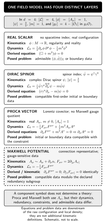
Four free models in four-dimensional Minkowski spacetime illustrate that a field symbol alone does not specify a theory: transformation and reality data, engineering dimensions, the local density and scales, derived equations, and admissible initial or boundary data occupy different layers. The equations are checked consequences shown for comparison rather than derivations developed on this page. The diagram is schematic and not to scale.

The table is the semantic counterpart of the diagram. “Problem data” names the additional data and compatibility conditions needed to select solutions; it does not assert existence or uniqueness.

Field	Kinematics and engineering dimension	Local dynamics	Derived equation and posed-problem data
Real scalar	A real field $\phi:M\to\mathbb R$ with $[\phi]=1$	$\frac12\partial_\mu\phi\,\partial^\mu\phi-\frac12m^2\phi^2$; reality is kinematic, while the kinetic and mass terms are dynamical	$(\Box+m^2)\phi=0$; specify compatible $(\phi,\dot\phi)$ on an initial slice or admissible boundary data
Dirac spinor	A complex four-component Dirac spinor with $\bar\psi=\psi^\dagger\gamma^0$ and $[\psi]=3/2$	$\frac{i}{2}[\bar\psi\gamma^\mu\partial_\mu\psi-(\partial_\mu\bar\psi)\gamma^\mu\psi]-m\bar\psi\psi$	$(i\gamma^\mu\partial_\mu-m)\psi=0$; specify compatible first-order initial or boundary data
Proca vector	A real Lorentz covector $A_\mu$, with $m\neq0$, $[A_\mu]=1$, and no Maxwell gauge identification	$-\frac14F_{\mu\nu}F^{\mu\nu}+\frac12m^2A_\mu A^\mu$	$\partial_\mu F^{\mu\nu}+m^2A^\nu=0$, which implies $\partial_\mu A^\mu=0$; data must satisfy the derived constraint
Maxwell potential	A real connection represented locally by $A_\mu$, with $[A_\mu]=1$ and admissible $A_\mu\mapsto A_\mu+\partial_\mu\alpha$	$-\frac14F_{\mu\nu}F^{\mu\nu}$; $F_{\mu\nu}=\partial_\mu A_\nu-\partial_\nu A_\mu$ is invariant	$\partial_\mu F^{\mu\nu}=0$, while $\partial_{[\lambda}F_{\mu\nu]}=0$ is kinematic; specify compatible data modulo the declared redundancy subgroup

The real-scalar density and the distinction between kinetic and interaction terms are introduced in Schwartz 2014, §§ 3.1–3.2, pp. 29–32. The Proca and Maxwell presentations, including the change in redundancy at zero mass, are compared in Schwartz 2014, §§ 8.2.2–8.2.4, pp. 114–120. The spinor field and Dirac density are constructed in Schwartz 2014, § 10.2.2, pp. 166–168.

The symmetrized Dirac density in the table is manifestly Hermitian. It differs from the compact form $\bar\psi(i\gamma^\mu\partial_\mu-m)\psi$ used in many treatments by a total divergence, so the two actions agree when the corresponding boundary contribution vanishes. The relevant integration-by-parts step and the compact spinor form appear in Schwartz 2014, § 3.2, p. 31; § 10.2.2, pp. 167–168. For the Dirac row, “complex spinor” is sufficient for the classical equation and transformation law. A variational or functional treatment that encodes fermionic statistics uses Grassmann-odd fields and must state whether $\psi$ and $\bar\psi$ are varied as independent variables; that structure belongs to the free-fermion and Grassmann pages.

The two vector rows show why component type is not physical content. Proca and Maxwell both use a symbol $A_\mu$, yet the mass term, redundancy, constraints, and eventual physical mode count differ. Conversely, the same physical model can be expressed in different variables. A configuration space must therefore be specified together with its transformations and equivalences, not inferred from notation.

Consistency checks

Three short checks catch most category and dimension errors on this page.

Reality and covariance. The scalar and vector densities are real Lorentz scalars under their declared field transformations. The displayed symmetrized Dirac density is manifestly Hermitian and Lorentz scalar. Its compact unsymmetrized form gives the same real action only when the total-divergence contribution is removed by the boundary behavior; in either form the adjoint $\bar\psi$ is essential, because $\psi^\dagger\psi$ alone is not a Lorentz-scalar mass term.

Dimensions. In $d=4$, every displayed density has dimension four. For example, $[F^2]=4$, $[m^2A^2]=2+2=4$, and $[\bar\psi\,\partial\psi]=3/2+1+3/2=4$.

Redundancy. Under an admissible $A_\mu\mapsto A_\mu+\partial_\mu\alpha$, the two extra derivatives in $F_{\mu\nu}$ cancel because partial derivatives commute. The Maxwell kinetic term is unchanged, whereas the Proca mass term is generally not. Whether a transformation with nontrivial boundary behavior is a redundancy or a physical symmetry requires the later boundary and charge analysis. This verifies the qualitative distinction without yet fixing a gauge or counting modes.

Common pitfalls

A point value is not a configuration. $\Phi^A(x)$ is one value of one section. Variations, actions, and boundary data act on entire configurations in $\mathcal F_{\mathrm{raw}}$.

A configuration is not a solution. Off-shell configurations are the inputs on which the action is defined. The equations select the on-shell subset; selected initial or boundary data then select solutions of a posed problem. A gauge theory adds the further distinction between a solution representative and its orbit under admissible redundancies.

Local does not mean ultralocal or automatically causal. Derivatives at the same point are local. Causal propagation and quantum spacelike compatibility require additional dynamical and structural hypotheses.

Engineering dimension is not full scaling dimension. The formulas above follow from canonical local terms. Interactions can produce anomalous dimensions, operator mixing, and scheme-dependent running; the distinction from canonical scaling is illustrated in Schwartz 2014, §§ 23.4–23.5, pp. 435–436.

Components do not count physical degrees of freedom. Constraints and redundancies can remove combinations of components, while reality conditions can relate them. The Proca–Maxwell comparison is the first warning, not the completed count.

Where the next questions go

Question	Continue with
Derive field equations and retain every surface term	The Action Principle and Field Equations
Decide which boundary data make the action differentiable	Boundaries, Variations, and Well-Posed Actions
Develop the Dirac model	The Dirac Field
Develop the massive vector model	The Proca Field
Develop Maxwell redundancy and physical content	The Free Maxwell Field and Gauge Redundancy
Treat global field geometry	Vector, Principal, and Associated Bundles and Bundle Connections, Curvature, Gauge Transformations, and Bianchi Identities
Determine gauge-invariant observable content	Gauge Fields, Redundancy, and Observable Content
Turn dimensional bookkeeping into a predictive expansion	Power Counting and Predictive Order

Check your understanding

Prompt	A satisfactory answer includes	Repair route
Name the data needed before $\mathcal L$ defines a classical local field model.	Spacetime, admissible field configurations with transformation/reality/redundancy data, the local density and parameters, and an allowed class of boundary or initial data	Re-read the model data
Distinguish $A_\mu(x)$, a raw Maxwell potential $A_\mu$, an on-shell potential, and a physical solution of a posed problem.	They are, respectively, a point value; a complete representative in $\mathcal F_{\mathrm{raw}}$; a representative satisfying Maxwell’s equations; and, after imposing the selected data, an orbit under the redundancy subgroup $\mathcal G_{\mathrm{red}}$	Re-read the first section and the comparison table
Derive $[\psi]=(d-1)/2$.	$[\bar\psi]=[\psi]$ and $[\bar\psi\,\partial\psi]=d$ give $2[\psi]+1=d$	Re-read Engineering dimensions and scales
Give one local action and one genuinely nonlocal quadratic action.	The local density uses a finite number of derivatives at one point; the nonlocal expression couples $x$ and $y$ through a kernel not supported on the diagonal	Re-read Locality and derivative order
Move the scalar comparison to $d=6$. What changes?	$[\phi]=2$, $[\lambda] = -2$ for a $\lambda\phi^4$ term, while the distinction among kinematics, dynamics, and problem data is unchanged	Re-run the displayed dimension equations
Where should one decide whether $\phi^4$ is important at low energy or whether two Maxwell potentials are globally gauge-equivalent?	Predictive power counting goes to Renormalization and EFT; global gauge equivalence goes to the bundle and symmetry treatments linked above	Use Where the next questions go

The central answer is now concrete: a field model is not specified by a component symbol or density alone. Its configuration space, local dynamical data, scales, and admissible problem data must be stated separately, and engineering dimensions provide the first consistency check. Variation of that data begins on The Action Principle and Field Equations.

References

• Harlow, Daniel, and Jie-qiang Wu. “Covariant Phase Space with Boundaries.” Journal of High Energy Physics 2020, no. 10 (2020): 146. DOI.
• Schwartz, Matthew D. Quantum Field Theory and the Standard Model. Cambridge: Cambridge University Press, 2014. DOI.
• Weinberg, Steven. The Quantum Theory of Fields. Volume I: Foundations. Cambridge: Cambridge University Press, 1995. DOI.