

Spacelike Compatibility and Local Observables
Spacelike compatibility is an algebraic locality test. In a theory with graded-local fields, homogeneous fields and satisfy
when the supports of and are spacelike separated. The bracket is a commutator unless both fields are odd, in which case it is an anticommutator. In the usual fermion-parity grading, the observable algebra is the even subalgebra, so observables localized in spacelike-separated regions commute in the ordinary sense. This condition is not a consequence of Lorentz covariance alone, and it does not say that spacelike correlations vanish.
Required background. Fields, Observables, and Interpolating Operators supplies the field–observable distinction used in the locality statement.
Helpful background. Quantum Fields as Operator-Valued Distributions supplies smearing and distributional support, while Hyperbolic Equations and Causal Propagators supplies causal support for the free-field check.
Spacelike-separated supports
Section titled “Spacelike-separated supports”With metric signature , two points are spacelike separated when
Two test-function supports are spacelike separated when this inequality holds for every and . It is not enough for their centers to be spacelike or for the functions to be evaluated at equal coordinate time.
For a homogeneous field, let denote its degree. The graded commutator is
Thus the locality bracket is
| Degrees | Spacelike bracket |
|---|---|
| even–even | |
| even–odd | |
| odd–odd |
Scalar and vector Bose fields are even; Dirac fields are odd. This grading statement is conditional: it states the locality property once the field grading is known. Deriving the relation between spin and grading is the separate spin–statistics theorem, with additional covariance, spectrum, positivity, vacuum, and domain hypotheses. The textbook field-level statements and their scalar and spinor realizations are developed in Schwartz 2014, § 12.6, pp. 219–223 and Weinberg 1995, § 5.1, pp. 198–200; § 5.2, pp. 201–205; and § 5.5, pp. 223–224.
Because fields are operator-valued distributions, the controlled statement is made after smearing. For the free scalar below, all commutators can be read on the common finite-particle domain. In a more general theory one must specify a common invariant domain, a quadratic-form interpretation, or a bounded algebraic formulation.
First application: the free scalar commutator
Section titled “First application: the free scalar commutator”Use the free real scalar normalization
Let and
Only the mixed – terms survive in the commutator:
This fixes the sign convention
Equivalently,
The four-momentum form makes proper-orthochronous Lorentz invariance manifest. It also shows distributionally that
Two equal-time checks fix the normalization:
Since differentiating the second field means , the second line gives
The mode calculation and its locality interpretation are given in Schwartz 2014, § 12.6, pp. 219–221.
Why the commutator vanishes outside the light cone
Section titled “Why the commutator vanishes outside the light cone”Let be spacelike. A proper orthochronous Lorentz transformation sends it to an equal-time vector,
Lorentz invariance of therefore reduces the calculation to
The two terms cancel under . Hence
This point-symbol calculation is shorthand for a distributional support statement:
For test functions define
Then
whenever and are spacelike separated. Hollands and Wald formulate the free field equation, causal propagator, and local smeared algebra at this level in Hollands and Wald 2015, § 2.1, pp. 9–12, PDF.
The derivation proves locality for this free scalar model. It does not prove that every Lorentz-covariant field theory is local; locality is a separate property or axiom that an interacting construction must satisfy.
The map below follows the support statement into its properly qualified locality conclusions. Inspect both the graded step and the separate admissibility check for physical observables.
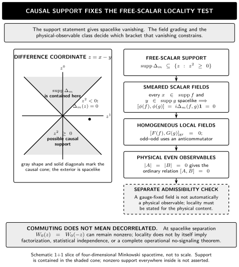
Causal support of the free-scalar Pauli–Jordan distribution yields vanishing smeared commutators for spacelike-separated supports. The general field statement is graded, while physical even observables commute ordinarily only after admissibility is established; the light-cone picture is a schematic 1+1 slice of four-dimensional Minkowski spacetime and is not to scale.
Read without the graphic: with the site’s metric, , so every spacelike cross-separation of and gives . Homogeneous fields use the graded bracket; even physical observables then obey the ordinary commutator relation, but a gauge-fixed field is not automatically such an observable. Vanishing commutators also do not imply vanishing correlations or statistical independence.
From graded fields to commuting observables
Section titled “From graded fields to commuting observables”Odd fields need not commute at spacelike separation. Instead, two spacelike-separated odd fields anticommute:
An even local combination contains an even number of odd factors. Moving one even combination past another produces an even number of minus signs, so the ordinary commutator vanishes. In graded notation, if and are physical even observables localized in spacelike-separated regions, then
This is why “fermion fields anticommute” does not mean that fermionic observables anticommute. The field algebra keeps the grading needed to construct charged or spinorial quantities; the observable algebra retains even, physically admissible content.
A gauge formulation requires another separation. Gauge-fixed fields can be useful representatives in an enlarged description, but their brackets do not by themselves establish locality of physical observables. Identifying the physical state space and observable content comes first; the free electromagnetic example is qualified at this level in Hollands and Wald 2015, § 3.3, pp. 55–58, PDF. Gauge-invariant, dressed, charged-sector, and cohomological constructions are handed to Gauge-Invariant and Dressed Observables.
A bounded region-level bridge
Section titled “A bounded region-level bridge”The bounded formulation avoids domain-sensitive products of unbounded fields. In the regular free Fock representation, let denote the self-adjoint Segal-field realization for real and define
Their multiplication law is
If the supports are spacelike separated, , and therefore
For a spacetime region , one may generate an algebra from with . Inclusion of regions then gives inclusion of these generated algebras, and spacelike-separated regions give commuting algebras. Abstract Weyl generators satisfy the same relations without being defined as exponentials of abstract field symbols; their algebra and local subalgebras are constructed in Fewster and Rejzner 2019, arXiv:1904.04051v2, §§ 4.1–4.2, PDF pp. 13–20. This is the bounded free-scalar seed of a local-net description, not a proof of all Haag–Kastler axioms. Precise choices of regions and completions, covariance, the vacuum representation, cyclicity, additivity, and spectral positivity belong to Haag–Kastler Nets and Locality.
Likewise, pairwise locality does not prove a local-to-global gluing theorem. Covers, derived colimits, and homotopy-coherent reconstruction belong to Weiss Descent and Local-to-Global Observables.
Commutation is not decorrelation
Section titled “Commutation is not decorrelation”The free vacuum two-point function is
Its antisymmetric part is the commutator:
At spacelike separation the two orderings agree, but each is generally nonzero. For , , and , angular integration followed by the standard radial transform gives
which is positive. The same spacelike transform appears in Weinberg 1995, § 5.2, p. 202, translated from his opposite metric convention. Its massless limit is
Thus expresses algebraic compatibility and order independence for spacelike-localized observables. It does not imply
nor does it by itself prove statistical independence, absence of entanglement, a tensor-product factorization, or a complete operational no-signaling theorem. Those require additional state, algebraic, and intervention assumptions; Fewster and Rejzner 2019, arXiv:1904.04051v2, § 5.2, PDF pp. 25–26, and § 7, PDF pp. 29–31 separates Einstein causality from stronger independence properties.
Scope and continuations
Section titled “Scope and continuations”The result has several precise boundaries:
- point fields are distributional notation; the controlled statement is smeared or algebraic;
- the free-scalar calculation verifies one model and does not derive locality from covariance;
- graded locality is stated after the field parity is known and does not prove spin–statistics;
- gauge-fixed field brackets are not automatically statements about physical observables;
- spacelike commutation does not erase vacuum correlations; and
- pairwise commutation does not supply the full local-net or descent structure.
The next chapter-local topic is Antiparticles and Charge-Conjugate Excitations. The broader physical principle and signaling cautions are developed in Microcausality and Relativistic Compatibility. The theorem connecting spin to statistics is The Spin–Statistics Connection.
Common pitfalls
Section titled “Common pitfalls”“Spacelike means equal time.” Equal time at distinct points is one spacelike configuration. A general spacelike pair can be brought to equal time by a Lorentz transformation, which is the step used in the scalar proof.
“A vanishing commutator means a vanishing correlator.” The commutator is the antisymmetric part of the two-point function. The symmetric part can remain nonzero, as the displayed result shows.
“Fermionic observables anticommute.” Odd field generators anticommute at spacelike separation. Physical even observables commute because their total grading is zero.
“Lorentz covariance guarantees locality.” Covariance constrains how fields transform. Spacelike graded commutation is an additional condition to impose or verify.
“A local gauge-fixed field is automatically a local observable.” Gauge fixing introduces useful representatives, often in an enlarged description. Physical locality must be stated for the physical observable content.
Check your understanding
Section titled “Check your understanding”-
Starting from the displayed mode expansion, derive and verify the two equal-time conditions.
Answer
The and terms commute. The term gives , while the reversed mixed term gives its negative with and exchanged. The delta function sets , leaving the displayed difference of plane waves with measure . At the integrand is odd under . Differentiating first and then setting yields ; the extra minus sign from restores the canonical bracket.
-
Why does the equal-time cancellation prove vanishing for every spacelike nonzero , but not for timelike ?
Answer
Every spacelike nonzero vector has a proper orthochronous Lorentz frame in which its time component is zero, and is invariant under that group. A timelike vector has no equal-time frame: its invariant square is positive, whereas every nonzero equal-time vector has negative square. The odd-integrand argument therefore applies exactly to the spacelike orbit.
-
How can be nonzero at spacelike separation when the commutator vanishes?
Answer
The commutator measures , not either term separately. At spacelike separation locality makes the two orderings equal. Their shared value can still be nonzero, so the vacuum may be correlated even though the corresponding observables are algebraically compatible.
References
Section titled “References”- Fewster, Christopher J., and Kasia Rejzner. “Algebraic Quantum Field Theory—an Introduction.” In Progress and Visions in Quantum Theory in View of Gravity, 1–61. Cham: Birkhäuser, 2020. DOI. Open PDF, arXiv:1904.04051v2.
- Hollands, Stefan, and Robert M. Wald. “Quantum Fields in Curved Spacetime.” Physics Reports 574 (2015): 1–35. DOI. Open PDF, arXiv:1401.2026v2.
- Schwartz, Matthew D. Quantum Field Theory and the Standard Model. Cambridge: Cambridge University Press, 2014. DOI.
- Weinberg, Steven. The Quantum Theory of Fields. Volume I: Foundations. Cambridge: Cambridge University Press, 1995. DOI.