Reflection Positivity within Osterwalder–Schrader Reconstruction

Reflection positivity tests a Euclidean hierarchy with a reflected positive-time quadratic form. If $F$ depends only on fields at $\tau>0$, the form pairs $F$ with its complex-conjugated image under $\tau\mapsto-\tau$ and must be nonnegative. Under an appropriate corrected Osterwalder–Schrader hypothesis package, that seminorm is one input to reconstructing a positive Lorentzian Hilbert space and positive-energy dynamics. It is not ordinary measure positivity, and by itself it does not reconstruct a QFT.

Required background. Euclidean Correlators and Schwinger Functions supplies the distributional Schwinger hierarchy, Euclidean source grammar, and the distinctions among covariance, measure, spectral, and reflected positivity.

Helpful background. The Källén–Lehmann Representation supplies the positive scalar spectral weights that make the free and generalized-free reflection kernels into Gram forms.

Euclidean time reflection defines a different quadratic form

Work with a real bosonic scalar hierarchy on Euclidean space and choose the reflection plane $\tau=0$. Let

$$\theta(\tau,\mathbf x)=(-\tau,\mathbf x), \qquad (\theta\phi)(\tau,\mathbf x)=\phi(-\tau,\mathbf x).$$

Let $\mathcal A_+$ be the finite polynomial functionals generated by fields smeared with test functions whose support lies strictly in $\tau>0$. Time reflection acts anti-linearly:

$$(\Theta F)[\phi] = \overline{F[\theta\phi]}, \qquad \Theta(cF)=\overline c\,\Theta F.$$

The Osterwalder–Schrader form is

$$(F,G)_{\mathrm{OS}} \equiv (F,G)_\theta \equiv \langle(\Theta F)G\rangle_E = \left\langle \overline{F[\theta\phi]}G[\phi] \right\rangle_E.$$

Reflection positivity is the statement

$$(F,F)_{\mathrm{OS}}\ge0 \qquad \text{for every }F\in\mathcal A_+.$$

If a positive Euclidean measure exists, the brackets are an ordinary integral. If only a Schwinger hierarchy is given, the same form is defined by distributional pairings. For

$$F[\phi]=\sum_{n=0}^{N}\phi^{\otimes n}(f_n),$$

with every $f_n$ supported where all Euclidean times are positive, one may write schematically

$$(F,F)_{\mathrm{OS}} = \sum_{m,n=0}^{N} S_{m+n}\!\left(\theta\overline{f_m}\otimes f_n\right) \ge0.$$

For a scalar symmetric hierarchy, reversing the reflected arguments does not change the value. For spinors, gauge fields, charged fields, or boundaries, the reflection operation includes additional index, adjoint, or geometric data and cannot be inferred from this scalar formula.

The restriction to $\tau>0$ is essential. It separates every reflected time from every unreflected time, so the reflection pairing itself creates no cross-plane coincidence. Contact terms already present among same-side insertions remain part of the declared hierarchy. If support reaches the reflection plane, boundary values and local terms require a separately declared domain.

Ordinary covariance positivity can fail the reflected test

Ordinary positivity asks for $\langle\overline F F\rangle_E\ge0$. Reflection positivity asks for $\langle\overline{F[\theta\phi]}F[\phi]\rangle_E\ge0$. The second does not follow from the first.

A Euclidean-invariant Gaussian near-miss makes the gap quantitative. Consider the momentum-space covariance

$$\widetilde C_2(p_E) = \frac{1}{(p_E^2+m^2)^2}, \qquad m>0.$$

It is a nonnegative Fourier multiplier, so its ordinary covariance form obeys

$$\int\frac{\mathrm d^d p_E}{(2\pi)^d} \frac{|\widetilde f(p_E)|^2}{(p_E^2+m^2)^2} \ge0.$$

At fixed spatial momentum, set $E=\sqrt{\mathbf p^2+m^2}$. The Euclidean-time kernel for a positive separation $s$ is

$$k_E(s) = \frac{e^{-Es}(1+Es)}{4E^3}.$$

For two distinct positive times, the reflected matrix has entries $M_{ij}=k_E(\tau_i+\tau_j)$ and determinant

$$\det M = -\frac{e^{-2E(\tau_1+\tau_2)}}{16E^4} (\tau_1-\tau_2)^2 <0.$$

The negative determinant forces one negative eigenvalue. Thus an ordinary positive, Euclidean-invariant Gaussian covariance can fail reflection positivity. The obstruction here is the repeated propagator pole; the example is a near-miss, not a candidate physical scalar theory. The general rational-propagator criterion likewise excludes repeated real poles Arici et al. 2018, Proposition 3.6 and Theorem 3.7, p. 8 (Open PDF).

The free scalar produces a finite Gram matrix

Now take the massive free scalar in finite spatial volume, retain one normalized Fourier mode with allowed spatial momentum $\mathbf p$, and set

$$E_{\mathbf p}=\sqrt{\mathbf p^2+m^2}>0, \qquad C_{\mathbf p}(\tau) = \frac{e^{-E_{\mathbf p}|\tau|}}{2E_{\mathbf p}}.$$

Choose finitely many Euclidean times $\tau_i>0$. Reflection sends the first insertion to $-\tau_i$, so the two-point reflection matrix is

$$\begin{aligned} K_{ij}(\mathbf p) &= C_{\mathbf p}(-\tau_i-\tau_j)\\ &= \frac{e^{-E_{\mathbf p}(\tau_i+\tau_j)}}{2E_{\mathbf p}} =v_i(\mathbf p)^*v_j(\mathbf p), \qquad v_i(\mathbf p)=\frac{e^{-E_{\mathbf p}\tau_i}}{\sqrt{2E_{\mathbf p}}}. \end{aligned}$$

Therefore, for arbitrary complex coefficients $c_i$,

$$\sum_{i,j}\overline{c_i}K_{ij}(\mathbf p)c_j = \frac1{2E_{\mathbf p}} \left| \sum_i c_i e^{-E_{\mathbf p}\tau_i} \right|^2 \ge0.$$

For two times the matrix is visibly rank one:

$$K(\mathbf p) = \frac1{2E_{\mathbf p}} \begin{pmatrix} e^{-2E_{\mathbf p}\tau_1} &e^{-E_{\mathbf p}(\tau_1+\tau_2)}\\ e^{-E_{\mathbf p}(\tau_1+\tau_2)} &e^{-2E_{\mathbf p}\tau_2} \end{pmatrix}, \qquad \det K=0.$$

The nonzero vector

$$n= \begin{pmatrix} e^{-E_{\mathbf p}\tau_2}\\ -e^{-E_{\mathbf p}\tau_1} \end{pmatrix}$$

has $n^\dagger Kn=0$. That null direction is not a negative norm; it says that these two Euclidean probes represent the same one-mode state up to their heat-kernel factors.

In infinite-volume notation, after a controlled spatial-volume limit, spatial smearing turns the same calculation into a Gram integral. For positive-time linear probes with spatial profiles $f_i$,

$$\begin{aligned} Q &= \int\frac{\mathrm d^{d-1}\mathbf p}{(2\pi)^{d-1}} \frac1{2E_{\mathbf p}} \left| \sum_i c_i e^{-E_{\mathbf p}\tau_i} \widetilde f_i(\mathbf p) \right|^2\\ &\ge0. \end{aligned}$$

This verifies a finite linear sector of the regulated free theory. It does not by itself prove positivity for every polynomial functional, every component of a continuum hierarchy, or an interacting measure. The page’s first application is deliberately an illustration, not the Osterwalder–Schrader theorem.

The free resolvent satisfies reflection positivity under the appropriate reflection and support hypotheses Jaffe and Ritter 2008, Theorem 1 and proof, pp. 2–3 (Open PDF). The rank-one fixed-momentum matrix above is the direct finite illustration of that structural result.

Positive spectral weights give the same mechanism

For a centered Hermitian scalar operator with a nonnegative Källén–Lehmann measure, and for smearings for which the spectral integral is finite, the reflected two-point matrix generalizes to

$$K_{ij}(\mathbf p) = \int_{[0,\infty)} \rho(\mathrm d\mu^2) \frac{e^{-E_{\mu,\mathbf p}(\tau_i+\tau_j)}} {2E_{\mu,\mathbf p}}, \qquad E_{\mu,\mathbf p}=\sqrt{\mathbf p^2+\mu^2}.$$

Hence

$$\sum_{i,j}\overline{c_i}K_{ij}c_j = \int_{[0,\infty)} \frac{\rho(\mathrm d\mu^2)}{2E_{\mu,\mathbf p}} \left| \sum_i c_i e^{-E_{\mu,\mathbf p}\tau_i} \right|^2 \ge0.$$

This is a sufficient two-point mechanism under the declared diagonal, positive-metric spectral assumptions. It is not a proof that an arbitrary Euclidean covariance has a positive spectral measure, and two-point positivity does not test incompatible higher Schwinger functions. A negative spectral component is a warning sign: suitable probes can expose a negative reflected norm even when some finite samples happen to pass.

Null directions motivate, but do not perform, reconstruction

A positive semidefinite form naturally suggests the null space and quotient

$$\mathcal N = \{F\in\mathcal A_+:(F,F)_{\mathrm{OS}}=0\}, \qquad \mathcal H_{\mathrm{candidate}} = \overline{\mathcal A_+/\mathcal N}.$$

This is only the physical picture. The exact construction must show that null vectors are orthogonal to all vectors, that the relevant observables and Euclidean transformations descend to the quotient, and that the completion has the required continuity and domain properties. Under the remaining hypotheses, positive Euclidean-time translations can induce a contraction semigroup $e^{-\tau H}$ with $H\ge0$; analytic continuation then supplies unitary real-time evolution. None of those conclusions follows from the displayed finite matrix alone.

The hypothesis map below should be read from left to right only conditionally: reflection supplies a candidate seminorm, while the other Osterwalder–Schrader inputs and the corrected theorem license the later arrows.

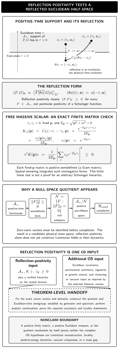
Schematic reflection-positivity mechanism and free-scalar check. At fixed spatial momentum, $K_{ij}=e^{-E_{\mathbf p}(\tau_i+\tau_j)}/(2E_{\mathbf p})$ is positive semidefinite. Quotienting zero-norm directions explains the candidate Hilbert-space step, but only a theorem-version-specific package of further Osterwalder–Schrader hypotheses licenses reconstruction. Arrows mark conditional mathematical dependence, not physical time evolution; the geometry is not to scale.

The figure’s relationships have the following text equivalent:

Region	Mathematical relation	Limit of the statement
Positive-time half-space	$F,G\in\mathcal A_+$ are paired after the first argument is reflected across $\tau=0$ and complex conjugated	reflection is an involution, not physical time evolution
Free finite kernel	$K_{ij}=e^{-E_{\mathbf p}(\tau_i+\tau_j)}/(2E_{\mathbf p})$ factorizes as a Gram matrix	a finite linear test is not a hierarchy-level proof
Null-space step	a positive semidefinite form motivates $\mathcal A_+/\mathcal N$ followed by completion	the exact domain, quotient, and descended operators require a theorem
Remaining OS input	covariance, symmetry, regularity or growth control, and the relevant clustering or vacuum condition join reflection positivity	the required package depends on the precise corrected theorem version
Theorem-level continuation	the full package supports the Hilbert-space, semigroup, analytic-continuation, spectrum, covariance, and locality constructions	reflection positivity or a positive finite matrix alone establishes none of these conclusions

Reflection positivity is one entry in the OS package

The original 1973 formulation labeled its Euclidean conditions E0–E4: distributional regularity or temperedness, Euclidean invariance, reflection positivity, permutation symmetry, and clustering. The same paper stated reconstruction directions from Euclidean to relativistic data and back Osterwalder and Schrader 1973, § 3, pp. 87–90 (Open PDF).

That original sufficiency claim needs its published correction. Osterwalder and Schrader later explained that a lemma used in the first proof was wrong, that E0–E4 as originally formulated were necessary but had not been shown sufficient, and that stronger regularity or growth alternatives repair the result Osterwalder and Schrader 1975, Introduction, pp. 281–283, and § IV.1, pp. 287–288 (Open PDF).

The durable division of labor is:

Input	Role in the reconstruction program	What reflection positivity does not supply
Distributional regularity and theorem-specific growth bounds	make the hierarchy and analytic continuation controllable	existence of boundary values or fields
Euclidean covariance	organizes translations and rotations before continuation	a Poincaré representation by itself
Permutation symmetry and hierarchy compatibility	encode the bosonic ordering relations needed for locality	locality from a two-point matrix
Reflection positivity	supplies the positive semidefinite time-reflected form	nondegeneracy, domains, or the remaining axioms
Clustering or the theorem’s vacuum condition	controls vacuum uniqueness and large-separation factorization	uniqueness from positivity alone

Different rigorous versions refine the first and last rows. This physical page therefore does not advertise E0–E4 as a universally sufficient five-item checklist.

What the reconstruction theorem still has to do

With an appropriate corrected hypothesis package, the downstream theorem must still:

1. define and complete the reflected quotient;
2. construct time and spatial translations and identify a nonnegative Hamiltonian;
3. continue Euclidean symmetry to a positive-energy Poincaré representation;
4. reconstruct operator-valued fields or equivalent observables on controlled domains;
5. recover locality and the Lorentzian Wightman distributions;
6. show that their Euclidean boundary values reproduce the starting hierarchy; and
7. state the theorem’s uniqueness and converse qualifications.

Reflection positivity directly addresses only the positive-seminorm part of that chain. Clustering, regularity, analyticity, locality, and uniqueness are not synonyms for it.

Common mistakes and failure modes

Passing one matrix is not proving the axiom. Every finite reflection matrix must be positive, and the full polynomial hierarchy must be compatible. A numerical eigenvalue above a tolerance tests only the chosen regulator, probes, and precision.

A positive covariance is not enough. The repeated-pole Gaussian above has a nonnegative Euclidean Fourier multiplier but fails the reflected form. The covariance must have the stronger reflection property.

Null vectors must not be retained as distinct physical states. Keeping them makes the would-be inner product degenerate and can make descended operators ill-defined. The quotient proof belongs to the rigorous treatment.

The reflection map is theory dependent. Fermions, gauge potentials, charged fields, boundaries, and lattice link variables require the correct adjoint, index transformation, physical subspace, and reflection plane. The scalar rule cannot be copied unchanged.

Complex weights need separate analysis. Chemical potentials, topological phases, sign-indefinite determinants, and complex cycles need not define an ordinary positive measure and may violate or modify the reflected test.

Check your understanding

1. Check anti-linearity

Why must $\Theta(cF)=\overline c\,\Theta F$ rather than $c\,\Theta F$?

Answer

The OS form must be conjugate-linear in its first argument and linear in its second, like a candidate Hilbert inner product. Without coefficient conjugation, $(F,F)_{\mathrm{OS}}$ need not be real and the Gram-matrix calculation would use $c_i c_j$ instead of $\overline{c_i}c_j$.

2. Find the free null direction

For the displayed two-time matrix, verify its determinant and identify a nonzero vector of zero norm.

Answer

The product of the diagonal entries equals the square of the off-diagonal entry, so $\det K=0$. The vector $(e^{-E\tau_2},-e^{-E\tau_1})^{\mathsf T}$ is orthogonal to $(e^{-E\tau_1},e^{-E\tau_2})^{\mathsf T}$ and therefore lies in the null space of the rank-one matrix.

3. Separate the positivity notions

Why does the repeated-pole covariance $\widetilde C_2(p_E)$ pass ordinary covariance positivity while failing reflection positivity?

Answer

Its Fourier multiplier is nonnegative, so the ordinary smeared covariance form is nonnegative. Reflection instead evaluates the two-time matrix $k_E(\tau_i+\tau_j)$; at distinct positive times its determinant is negative. The two quadratic forms test different pairings.

4. Locate the theorem boundary

If all tested free-scalar reflection matrices are positive, what remains before claiming a reconstructed Lorentzian QFT?

Answer

One needs the complete hierarchy, a corrected regularity or growth package, Euclidean covariance, symmetry, clustering or the relevant vacuum condition, the quotient and completion, controlled analytic continuation, and reconstruction of positive-energy local fields. Those results belong to the Mathematical QFT treatments linked below.

Where to continue

• Osterwalder–Schrader Axioms and Reflection Positivity states the exact hypothesis packages and tests their variants.
• Reflection Positivity and Hilbert-Space Reconstruction constructs the null quotient, completion, semigroup, and positive Hamiltonian.
• Osterwalder–Schrader Reconstruction develops the full reconstruction theorem and its qualifications.
• Counterexamples, Nonconverses, and Hypothesis Stress Tests supplies systematic failures when a theorem hypothesis is weakened.

References

• Arici, Francesca, Daniel Becker, Chris Ripken, Frank Saueressig, and Walter D. van Suijlekom. “Reflection Positivity in Higher Derivative Scalar Theories.” Journal of Mathematical Physics 59 (2018): 082302. DOI. Open PDF.

• Jaffe, Arthur, and Gordon Ritter. “Reflection Positivity and Monotonicity.” Journal of Mathematical Physics 49 (2008): 052301. DOI. Open PDF.

• Osterwalder, Konrad, and Robert Schrader. “Axioms for Euclidean Green’s Functions.” Communications in Mathematical Physics 31 (1973): 83–112. DOI. Open PDF.

• Osterwalder, Konrad, and Robert Schrader. “Axioms for Euclidean Green’s Functions II (with an Appendix by Stephen Summers).” Communications in Mathematical Physics 42 (1975): 281–305. DOI. Open PDF.