

Canonical–Functional Crosswalk for Regulated Systems
Canonical and functional calculations agree in the example below because they are two exact representations of the same finitely regulated oscillator system. For finitely many massive scalar modes sampled at finitely many Euclidean times, the exact transfer kernel and the vacuum wave functions define a normalized finite Gaussian integral. Its covariance is precisely the Euclidean time-ordered vacuum two-point function computed with creation and annihilation operators. The equality requires the same regulator, Hamiltonian and ordering, operator domain, state, boundary data, normalization, source, observable, and prescription. It is not a universal equivalence theorem for canonical and functional formulations of QFT.
Required background. Time Slicing and Transition Amplitudes supplies the normalized kernel construction and its ordering data. Gaussian Fields and Sources supplies finite Gaussian source derivatives and inverse-kernel checks. Quantizing the Real Scalar Field supplies the finite-mode oscillator algebra and selected vacuum.
Helpful background. Boundaries and State Preparation distinguishes a fixed-endpoint kernel from the vacuum matrix element obtained by attaching and integrating boundary wave functions.
The comparison fixes one finite oscillator system
Section titled “The comparison fixes one finite oscillator system”Let a spatial regulator retain real orthonormal scalar modes with strictly positive frequencies . A finite box, boundary condition, and mode cutoff are included in . We use natural units, set the oscillator masses to one by the choice of canonical coordinates, and assume so that no periodic zero-frequency mode occurs.
We take the standard self-adjoint oscillator Hamiltonian on the canonical Hilbert space, with the following chosen invariant core:
Here , acts by multiplication, and on . The regulated Hamiltonian has the following differential expression on that core:
Euclidean sample times are for , with , , and . Instead of assuming a continuum product measure, the functional side will contain only the real coordinates . Each interval uses the exact matrix element ; no Trotter error is hidden in the main match. Sources couple directly as . If a continuum source is later sampled on the grid, its relation to requires a declared quadrature rule.
The choices that must coincide are:
| Datum | Canonical choice | Functional choice and check |
|---|---|---|
| System | The same real modes and frequencies | The same coordinates and quadratic kernel; spectra agree mode by mode |
| Algebra and domain | , , and on the stated core | Coordinate integrations over with no omitted boundary term |
| Ordering | Euclidean time ordering generated by | Exact transfer kernels, or a separately declared ordered short-step approximation |
| State and boundary | The normalized vacuum | The same ground-state wave function at both endpoints, integrated once each |
| Normalization | Normalized vacuum matrix elements | Every kernel and endpoint factor retained, so the zero-source measure integrates to one |
| Source and observable | Ordered products of the retained | Derivatives with respect to the direct source |
| Prescription and limits | Euclidean decay in the chosen vacuum; fixed | The same decay and fixed ; no spatial cutoff removal inferred |
This is a comparison record, not extra dynamics. A disagreement in any row means that the two calculations are not yet computing the same object.
Canonical operators give the vacuum covariance
Section titled “Canonical operators give the vacuum covariance”For one retained mode, suppress the label and write
Euclidean evolution gives
For , only contributes. Euclidean time ordering therefore yields
For all retained modes, define
The canonical vacuum two-point function is then the finite sum
Every term is an ordinary oscillator matrix element. The spatial cutoff makes the sum finite, and makes the selected Gaussian vacuum normalizable.
Exact Euclidean kernels give a finite Gaussian chain
Section titled “Exact Euclidean kernels give a finite Gaussian chain”For the same one-mode Hamiltonian, the normalized ground-state wave function and energy are
The exact Euclidean transfer kernel over one interval is
It is the coordinate matrix element of , with the endpoint values and normalization shown explicitly (Zinn-Justin 2021, § 2.3, pp. 24–25). Attach the same vacuum at both endpoints and integrate every sampled coordinate once:
This is a finite positive measure. Its normalization is an operator identity:
Coordinate resolutions, fixed endpoints, boundary states, and the ordering encoded by the transfer operator are the ingredients that connect canonical matrix elements to functional representations (Weinberg 1995, §§ 9.1–9.4, pp. 378–398). Here the exact kernel makes the bridge finite-dimensional at every stage.
The structure becomes transparent after setting
The joint measure factorizes into a stationary initial density and normalized conditional densities:
where
and
The factors follow by completing the square in the exact kernel. They exhibit the boundary preparation, all normalization constants, and the finite-dimensional integration domain without introducing a symbol such as .
The finite functional covariance matches mode by mode
Section titled “The finite functional covariance matches mode by mode”The conditional Gaussian can be represented as
with the independent of earlier coordinates. The initial density has , so the variance remains stationary:
For , repeated conditioning gives
Thus
for every , every , and every pair of sampled times. There is no time-slicing limit in this equality because each interval used the exact transfer kernel.
The normalized finite source integral is consequently
and
If a continuum source is sampled by , then . For example, trapezoidal sampling has and at interior nodes. Therefore
The direct finite source needs no continuum quadrature; differentiating with respect to as though it were would compare different source conventions.
For the multimode figure below, we use the compact definitions
Taking the product of these normalized chains over gives the declared free-scalar result:
with both sides equal to the same finite mode sum displayed above. The usual Euclidean oscillator source functional and its vacuum covariance are obtained by the same Gaussian calculation (Zinn-Justin 2021, § 2.6, pp. 30–31).
The inverse-kernel contact check closes the derivation
Section titled “The inverse-kernel contact check closes the derivation”The finite chain itself supplies an independent Gaussian check. Its exponent can be written as , up to the normalized constant factors, with tridiagonal precision matrix
All other entries vanish. Substituting gives
For an interior row, the equality follows from
which vanishes for and equals one for ; the two endpoint rows work because the vacuum wave functions supplied the endpoint entries of . Omitting those wave functions changes the inverse problem.
At continuous Euclidean time, the same invariant check is
For , its restriction also satisfies the vacuum endpoint conditions
These are the continuous counterparts of the two special endpoint rows of ; the differential equation alone does not select this inverse.
The derivative jump is
Mode by mode, this tests the oscillator normalization and equal-time commutator. For the field, the spatial sum reconstructs the regulated identity kernel
not an unregulated spatial delta distribution.
The matched data make the equality conditional
Section titled “The matched data make the equality conditional”Read the diagram as a data-matching test: trace the operator and Gaussian routes to their common regulated covariance, then inspect every equality gate and the dashed list of excluded claims.
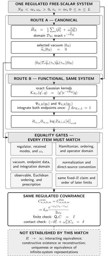
For a fixed spatial regulator and a finite set of Euclidean samples, the solid routes are exact because every interval uses the same transfer operator. The shared endpoint is the covariance and its contact equation. The dashed boundary marks claims not established by this comparison: spatial regulator removal, interacting equivalence, reconstruction, or uniqueness of infinite-system representations. The diagram is schematic and not to scale.
Read the two routes from top to bottom. Route A ends at . Route B uses the exact Gaussian kernels, integrates both endpoint wave functions once over , and ends at . Its normalization is . The gates require equality of the regulator and spectrum; Hamiltonian, ordering, and operator domain; vacuum, endpoint data, and integration domain; normalization and source convention; observable and prescription; and fixed- claim and limit order. Only then do the routes yield the common covariance, whose independent checks are and . The dashed box lists the excluded continuum, interacting, reconstruction, and representation claims. Open the SVG alone for scalable zoom and pan.
A mismatch in any defining datum stops the comparison
Section titled “A mismatch in any defining datum stops the comparison”The exact calculation has a sharp domain of validity:
| Mismatch | What changes |
|---|---|
| Remove the endpoint vacuum wave functions | The finite Gaussian has different endpoint rows and no longer computes the vacuum matrix element |
| Identify the two endpoints and integrate once | The object becomes a trace; at finite Euclidean extent it gives a thermal covariance |
| Replace the exact kernel by a short-step action | Equality acquires the product-formula error and ordering convention of that approximation |
| Change the spatial cutoff or boundary condition | The frequency list and regulated identity kernel change, so the systems differ |
| Set some | The ground-state Gaussian and covariance cease to exist in that direction |
| Couple but differentiate as though the source were | The quadrature weights spoil the comparison |
| Use a Lorentzian bulk action without a contour or | The oscillatory Gaussian and its inverse are not yet specified |
| Use a constrained or gauge-redundant system | The unconstrained coordinate measure and oscillator domain no longer apply |
For the matched Feynman vacuum prescription, define . The one-mode Lorentzian result is
Its contact term differs from the Euclidean one. A retarded, advanced, thermal, or fixed-boundary inverse has another boundary condition even when the denominator looks the same. The time-slice spacing controls a product approximation when one is used; selects a Lorentzian boundary value. They are not the same limit.
For nonquadratic momentum dependence, coordinate-dependent kinetic terms, momentum sources, or composite insertions, the finite-slice ordering and momentum integrations must be carried explicitly. Only suitable nonsingular quadratic momentum dependence reduces those integrations to Gaussian determinants. For an interacting or infinite system, agreement of one regulated two-point function does not construct the limit, identify representations, or prove reconstruction.
Common pitfalls
Section titled “Common pitfalls”Matching only the differential operator. Boundary conditions, state, and prescription select its inverse. Equal denominators do not identify Feynman, retarded, thermal, Dirichlet, and vacuum-projected kernels.
Comparing a kernel with a vacuum expectation value. A fixed-endpoint kernel leaves and unintegrated. The vacuum matrix element attaches and and integrates both endpoints exactly once.
Cancelling normalization before the objects match. Determinants and kernel prefactors cancel in a normalized source ratio only when the kernel, boundary data, and reference measure are unchanged. The finite chain above keeps every factor until its integral is demonstrably one.
Forgetting which source is differentiated. A direct discrete source and a quadrature-sampled continuum source differ by . Source derivatives must be translated before their correlators are compared.
Promoting fixed-regulator agreement to universal equivalence. The proof covers a finite free oscillator system and a selected observable. Spatial cutoff removal, interacting existence, reconstruction, and representation comparison require separate hypotheses and theorems.
Check your understanding
Section titled “Check your understanding”-
Starting from the conditional density , verify its mean, variance, and stationary density.
Solution
Completing the square shows that is Gaussian with mean and variance . If has variance , then has variance . Its mean remains zero, so is stationary.
-
Multiply one interior row of by .
Solution
For , set . The three terms are proportional to . For , the bracket is times ; the prefactor makes the result one.
-
Apply to , including the origin.
Solution
Away from the origin the two terms cancel. The first derivative jumps from on the left to on the right, so its jump is . Distributionally, therefore contributes .
-
Replace the two endpoint vacuum wave functions by periodic identification and one integration over that common coordinate. What object is computed?
Solution
Removing the compensating factor , the integrations form rather than . If that factor is retained from the displayed vacuum measure, the result is ; it cancels in a normalized source ratio. In either convention, normalized insertions give a thermal correlator at inverse temperature (with units restored), not the exact vacuum correlator at finite .
-
Set one retained frequency to zero. Which steps fail first?
Solution
The proposed ground-state wave function becomes nonnormalizable, the stationary density disappears, and the covariance diverges. The zero mode needs a separate infrared definition before either side of the comparison is meaningful.
Where this crosswalk leads
Section titled “Where this crosswalk leads”- Scalar Propagators, Ordered Correlators, and Sources distinguishes the Feynman, retarded, advanced, and Wightman kernels that a common denominator does not distinguish.
- The Generating Functional develops normalized source derivatives beyond this finite free match.
- Wick Rotation and Analytic Continuation states the analytic and contour hypotheses needed to relate Euclidean and Lorentzian objects.
- Lattice Regulators and Target Continuum Theories develops spatial cutoff removal and tests of the continuum limit.
- Equivalence, Uniqueness, and Comparison Notions distinguishes regulated agreement from unitary equivalence, quasiequivalence, reconstruction, and other framework-level claims.
References
Section titled “References”- Weinberg, Steven. The Quantum Theory of Fields, Volume I: Foundations. Cambridge University Press, 1995. doi:10.1017/CBO9781139644167.
- Zinn-Justin, Jean. Quantum Field Theory and Critical Phenomena. 5th ed. Oxford University Press, 2021. doi:10.1093/oso/9780198834625.001.0001.