

One-Particle States: Mass, Spin, and Relativistic Normalization
In a positive-energy, Poincaré-covariant theory on four-dimensional Minkowski spacetime, a sharp stable particle species is represented by an invariant Hilbert subspace carrying an irreducible unitary representation of the appropriate cover of the connected Poincaré group. Its momentum orbit fixes the mass. The subgroup that leaves one standard momentum fixed—the little group—supplies spin for a massive species or helicity for an ordinary massless species. An invariant measure on that orbit then turns generalized momentum kets into normalizable wave packets.
Those three ingredients answer the defining question: a relativistic one-particle state is a wave packet on a positive-energy mass shell, valued in a little-group representation and normalized with the corresponding invariant measure. This statement presupposes that a sharp one-particle subspace exists. It does not turn a resonance or an infraparticle into such a state, and it does not construct interacting in/out states.
Helpful background. Lorentz-Field and Poincaré-Particle Representations supplies the representation-theory machinery, while Hilbert Spaces, Completion, and the Riesz Representation Theorem distinguishes generalized eigenkets from Hilbert-space vectors.
The sharp-mass one-particle setting
Section titled “The sharp-mass one-particle setting”We assume:
- exact covariance under the connected proper-orthochronous Poincaré group, lifted to its cover when half-integer spin is present;
- a positive-energy representation with a distinguished sharp-mass one-particle subspace;
- the site conventions , , and ; and
- natural units, with all factors of kept explicit.
Parity and time reversal are not included unless stated separately. The massless discussion is restricted to finite-helicity representations; continuous-spin representations are outside the page’s scope.
Vacua, States, and Representations places the chosen particle-sector representation in its broader state-and-representation context without being required for the construction below.
What counts as a one-particle sector?
Section titled “What counts as a one-particle sector?”Let carry the positive-energy Poincaré representation and let be the invariant one-particle sector for a species . A generalized simultaneous eigenket of the translation generators satisfies
Here distinguishes species or repeated copies of the same Poincaré representation. The discrete label describes a basis in the little-group representation. For fixed , the Hilbert closure of square-integrable superpositions of these generalized kets furnishes an irreducible representation. A full one-particle space containing several species is generally a direct sum .
The word “particle” here is representation-theoretic. A stable bound state can define a one-particle species even though it is composite, and distinct species can share the same mass and spin. Conversely, the sharp ket is not a normalizable vector: its norm contains a momentum delta distribution. Normalizable vectors are wave packets built from these kets. Weinberg 1995, § 2.5, pp. 63–65 gives this definition and explicitly notes that elementary versus composite is not part of it.
Only in a setting with a suitable number operator—most transparently a free Fock representation—does “one particle” also mean an eigenvalue-one sector. The Poincaré definition does not assume such an operator.
From a momentum orbit to the little group
Section titled “From a momentum orbit to the little group”Choose a standard momentum on a positive-energy orbit and a standard Lorentz transformation satisfying . For a Lorentz transformation , the combination
leaves fixed and therefore belongs to its little group. In the covariant normalization adopted below, the one-particle transformation law can be written
The matrices are unitary. Their unitarity preserves the finite-dimensional or helicity indices, while invariance of the mass-shell measure preserves the momentum part of a packet norm. The choice of standard transformations changes the momentum-dependent basis, not the representation’s invariant content. The induced-representation proof belongs to Mathematical Methods; the construction and its normalization are developed in Weinberg 1995, § 2.5, pp. 63–68.
Massive spin and massless helicity
Section titled “Massive spin and massless helicity”The translation and Lorentz generators define the Pauli–Lubanski vector
Here are the Lorentz generators, and the spatial rotation generators are with .
Together, and classify the familiar massive irreducible representations. The massless finite-helicity case needs additional little-group data because both Casimirs vanish. The connected Poincaré group and its cover derives these invariants from the Poincaré algebra.
| Feature | Massive species | Massless finite-helicity species |
|---|---|---|
| Momentum orbit | , | , |
| Standard momentum | , | |
| Little group | , lifted to | , with its translation-like part acting trivially |
| Invariant label | spin | helicity |
| Basis at fixed momentum | one component for each irreducible helicity | |
| Pauli–Lubanski relation | , hence |
For , a rest frame exists. At , the declared conventions give
The little group is the rotation group, and its irreducible unitary representations have . The spin projection depends on a chosen basis and is mixed by Wigner rotations; the total spin is invariant.
For , no rest frame exists. Choosing a standard null momentum gives the little group . In a finite-helicity representation its translation-like subgroup acts trivially, while the rotation about the momentum direction acts by a phase. Its label is the eigenvalue of the helicity operator:
At the standard null momentum , trivial action of the two translation-like little-group generators makes the transverse components of vanish. The remaining rotation generator gives
Lorentz covariance extends this relation to every momentum on the orbit. Helicity is therefore invariant under the connected proper-orthochronous group. Opposite helicities are separate irreducible representations of that connected group; parity relates them only if parity is also a symmetry. If the translation-like part of acts nontrivially, one obtains continuous-spin rather than finite-helicity representations. Those representations are mathematically distinct, not an extra polarization hidden in the table. Weinberg 1995, § 2.5, pp. 68–74 develops the massive and massless little groups and the finite-helicity restriction.
This also explains why one should not call helicity “massless spin” without qualification. For every finite helicity, , so the Casimirs alone do not determine . Nor is a massive spin- representation converted into a massless helicity representation by merely setting in a formula: the little group and the number of polarization states change.
Deriving the invariant mass-shell measure
Section titled “Deriving the invariant mass-shell measure”For a massive orbit set
The four-dimensional measure , the scalar , and the sign of are preserved by proper-orthochronous Lorentz transformations. Therefore
The second line follows from
because retains only the positive-energy root. Thus
is Lorentz invariant on the future mass shell. The same formula applies at with away from the cone’s apex. The factor is forced by restricting the invariant four-dimensional measure; the factor is our Fourier-normalization choice. Coleman 2019, § 1.2, pp. 9–10 gives this derivation and its relation to relativistically normalized kets.
Relativistic normalization and wave packets
Section titled “Relativistic normalization and wave packets”Fix one species of mass and suppress in this section. We choose the covariant sharp-ket normalization
Its reciprocal measure appears in the resolution of the identity on the one-particle space:
This is not the identity on the vacuum and multiparticle sectors. It is the spectral resolution on the fixed species sector , understood distributionally. For several species, one takes the direct sum and uses each species’ own mass-shell measure. The normalization check is the cancellation
A Hilbert-space vector is a packet
with norm
The positive measure makes the norm manifestly positive. Under a Lorentz transformation, the momentum argument moves along the same orbit and the components rotate by . Invariance of and unitarity of therefore preserve the packet norm. This is the physical check that the state normalization and transformation law have been paired correctly.
The map below gathers the orbit, little-group label, invariant measure, sharp-ket normalization, completeness relation, and packet norm into one chain. Inspect where the massive and massless branches differ and where their normalization data rejoin.
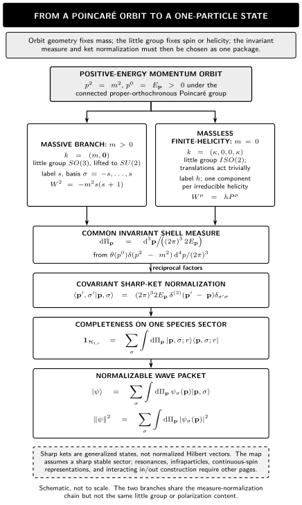
A positive-energy Poincaré orbit fixes the mass, its little group fixes spin or finite helicity, and the invariant shell measure must be paired reciprocally with covariant sharp-ket normalization. The branches share the measure–normalization chain but not their little groups or polarization content; the map assumes a sharp stable one-particle sector and is schematic, not to scale.
Read without the graphic: the massive orbit has little group lifted to and , whereas an ordinary massless finite-helicity orbit has with trivial translation-like action and . In both cases cancels the reciprocal factor in the covariant ket norm, giving the displayed completeness and packet formulas. Resonances, infraparticles, and continuous-spin representations are outside this chain.
For a normalized packet, the momentum-space probability measure is
not unless the wave function has first been rescaled to a different convention.
A normalization crosswalk
Section titled “A normalization crosswalk”One may instead use delta-normalized kets
for which
Then completeness uses . Equality of the two packet expansions requires
Even a scalar delta-normalized sharp ket acquires a boost Jacobian:
Neither convention is more physical. Mixing pieces of the two is the error: one cannot keep delta-normalized kets, the invariant measure, and the transformation law with no Jacobian simultaneously.
There is also a source-convention translation. Weinberg’s treatment orders the three spatial components before the time component, uses the mostly-plus metric, and adopts a delta-normalized basis. Thus its massive standard momentum becomes our , its null momentum becomes our , and its equation becomes . Applying the ket rescaling above then reproduces our normalization formulas. The momentum orbit, stabilizer group, mass and spin or helicity labels, and packet norm are invariant checks of this translation; the signature-dependent Casimir formulas must be translated with the metric. Weinberg 1995, § 2.5, pp. 63–74 is the source treatment being translated.
First application: a massive scalar
Section titled “First application: a massive scalar”For a massive scalar, and the little-group representation is trivial. Its one-particle space is
The Lorentz action on covariantly normalized sharp kets is simply
In the free real-scalar Fock realization, use the convention
The covariantly normalized generalized ket is then
Indeed, the creation-operator commutator gives
where the delta distribution permits replacing by . The corresponding normalized packet is
This is the positive-frequency scalar space used in the standard vacuum representation; it is not the vacuum line . The free creation operator realizes the packet inside Fock space, but tensor powers, statistics, and the full creation-operator organization belong to the next page. The relativistic spin-zero state normalization appears in Coleman 2019, § 1.2, pp. 6–10; the Fock and free-scalar realizations are constructed in Coleman 2019, § 2.4, pp. 26–30; §§ 3.3–3.4, pp. 38–44.
For the massless scalar comparison, set so that . The particle has helicity , and the same invariant-measure and packet-normalization formulas apply. Kinematically, however, its little group is now rather than . A nonzero-helicity massless particle is likewise described by a packet on the future light cone, but each irreducible helicity carries its own little-group phase. The scalar little-group and polarization comparison is simple; infrared and zero-mode limits remain separate questions. Higher-spin massless limits require additional dynamical and often gauge-theoretic analysis.
What the labels do—and do not—decide
Section titled “What the labels do—and do not—decide”Mass, spin or helicity, and internal quantum numbers distinguish a particle species only after the theory and representation are specified. The Poincaré labels alone do not decide:
- whether two copies with identical and are the same species;
- whether a local field has a nonzero matrix element with the particle;
- which finite-dimensional Lorentz representation should be used for field components;
- whether multiparticle states are bosonic or fermionic;
- whether locality, the spin–statistics connection, or CPT holds;
- whether an interacting theory actually has isolated stable-particle states; or
- whether scattering wave operators exist or are asymptotically complete.
In particular, a Lorentz index on a field is not a particle spin label. Field components transform in finite-dimensional, generally nonunitary Lorentz representations; physical state vectors transform in unitary Poincaré representations. Their relation is a question about vacuum-to-particle matrix elements and constraints, not an identification.
Boundaries and continuations
Section titled “Boundaries and continuations”- Vacua, States, and Representations supplies the state and Hilbert-space setting in which a one-particle subspace may be selected.
- Multiparticle States, Statistics, and Fock Organization takes and its normalization as inputs and builds symmetric or antisymmetric sectors.
- Fields, Observables, and Interpolating Operators explains how a field can overlap this particle sector without being identical to it.
- Lorentz Field Representations and Poincaré Particle Representations develops the induced-representation machinery and the comparison between field and particle representations.
- Resonances, Infraparticles, and Limits of Particle Language determines when the sharp one-particle assumption fails.
- In and Out States, S- and T-Matrix Normalization, and LSZ Reduction develop interacting asymptotic states and scattering conventions.
Common pitfalls
Section titled “Common pitfalls”“A sharp momentum ket is a physical normalized state.” It is a generalized eigenket with a delta-distribution norm. A physical state in is a square-integrable packet.
“The measure is Lorentz invariant.” It is invariant under spatial rotations, not boosts. On the positive-energy mass shell, is invariant.
“Ket normalization and integration measure are independent choices.” They are reciprocal parts of the completeness relation. Changing one requires changing the wave function and transformation law as well.
“Spin is the number of components of a covariant field.” Particle spin comes from a unitary little-group representation. Field components belong to a different Lorentz representation and may contain constraints, gauge redundancy, or overlap with several particle sectors.
“A massive spin multiplet has the same states after setting .” The little group changes from to . A controlled massless limit can require gauge symmetry or other dynamics and cannot be inferred from the mass-shell equation alone.
“Mass and spin uniquely name a particle.” They classify a Poincaré representation, not every repeated copy or internal quantum number. Several species can share the same Poincaré labels.
Check your understanding
Section titled “Check your understanding”-
Starting from the four-dimensional shell distribution, derive and explain which root is removed by .
Answer
Factor into its two simple roots. The delta-function change-of-variables rule gives one term at and one at , each with Jacobian . The step function removes the negative-energy root. Since the original four-dimensional expression is Lorentz invariant under the proper-orthochronous group, the resulting shell measure is invariant.
-
Why does not determine a massless particle’s helicity, and what extra datum does?
Answer
In every finite-helicity massless representation, . Because , this implies for every value of . The one-dimensional rotation representation of the massless little group supplies the helicity phase and therefore distinguishes the representations.
References
Section titled “References”- Coleman, Sidney. Lectures of Sidney Coleman on Quantum Field Theory. Edited by Bryan Gin-ge Chen, David Derbes, David Griffiths, Brian Hill, Richard Sohn, and Yuan-Sen Ting. Singapore: World Scientific, 2019. DOI.
- Weinberg, Steven. The Quantum Theory of Fields. Volume I: Foundations. Cambridge: Cambridge University Press, 1995. DOI.