

Poles, Cuts, Thresholds, and Stable Particles
In a positive-metric scalar vacuum two-point function, an isolated atom in the Källén–Lehmann measure produces a simple pole on the physical sheet, while continuous spectral support from produces a discontinuity and, in the infinite-volume limit, a cut beginning at the threshold. The endpoint is not a particle: it is the lightest invariant mass available to a continuum in that operator channel. An isolated pole with nonzero overlap identifies a stable one-particle spectral sector, but it does not by itself establish LSZ limits, asymptotic completeness, or infrared suitability.
The derivation below concerns the complexified invariant of a vacuum two-point function. It does not derive second-sheet resonance poles, general amplitude singularities, or dispersion bounds.
Required background. The Källén–Lehmann Representation supplies the positive scalar measure, its atom–continuum split, the common prescription, and the local-polynomial qualification used here.
Helpful background. Spectra, Resolvents, Spectral Measures, and Functional Calculus supplies the spectral-transform language. Branches, Sheets, Analytic Continuation, and Monodromy fixes the sheet and continuation vocabulary, while Boundary Values, Discontinuities, and Dispersion Integrals supplies the boundary-value and discontinuity tools.
The physical-sheet singularity dictionary
Section titled “The physical-sheet singularity dictionary”Write the invariant-mass variable in the spectral integral as and complexify the external invariant to . For the simplest channel with one isolated scalar state below a continuum,
When the continuum integral is ultraviolet convergent without subtractions, separate the site’s numerator- convention by defining the spectral transform
Here is an allowed local polynomial. When the chosen time-ordered extension has no local term, set . When the displayed integral is not ultraviolet convergent, replace it by the preceding page’s -subtracted kernel; that kernel defines the same nonlocal analytic data up to a polynomial. Polynomials are entire, so they cannot create an isolated pole, a threshold branch point, or a discontinuity.
The physical Feynman correlator is the upper boundary value
The physical sheet is the branch reached from spacelike , with the continuum cut chosen along . The prescription approaches its upper rim. For any function with two boundary values, this page uses
These choices fix the signs in the entire dictionary.
An isolated spectral atom gives a simple pole
Section titled “An isolated spectral atom gives a simple pole”Near , the continuum term is analytic because its support begins a positive distance away at . Therefore
with holomorphic in a neighborhood of . It follows immediately that
The positive quantity is the residue of . In the site’s convention the residue of itself is , not a positive real number.
The atom came from a nonzero vacuum-to-one-particle matrix element, so the pole identifies an exact one-particle mass sector seen by . Isolation below prevents this state from dissolving into the displayed continuum. The state can be a bound state; no field with the same name need appear in a Lagrangian. Conversely, if one operator has zero overlap, its two-point function can miss a particle that another operator detects. Schwartz 2014, § 24.3, pp. 471–474 and Weinberg 1995, § 10.2, pp. 430–434 derive the one-particle pole from intermediate-state insertion and explicitly include composite or bound states. Weinberg uses a mostly-plus metric, so his maps to the site’s ; the pole order and intermediate-state interpretation are unchanged.
Continuum support gives a threshold cut
Section titled “Continuum support gives a threshold cut”At a regular point where the continuum has an ordinary density, the Sokhotski–Plemelj boundary values give
Subtracting the two rows yields the sign-sensitive result
The second sign differs because . It is therefore unsafe to copy an imaginary-part formula written for a propagator with another overall normalization. The discontinuity is the convention-stable check here: the polynomial cancels, and
on the continuum. For a general measure, this statement is understood distributionally rather than as a pointwise formula.
The lower endpoint is a threshold. When, for example, a four-dimensional two-body -wave density has
the transform contains a corresponding square-root nonanalyticity at up to analytic terms. Continuing around that endpoint changes branch, so is a branch point and the ray is a convenient physical cut. Other channel quantum numbers, spacetime dimensions, partial waves, or singular form factors can change the threshold exponent. Continuum support fixes the discontinuity; it does not make the endpoint itself a particle.
The pole-and-cut sheet map
Section titled “The pole-and-cut sheet map”The upper panel of the figure summarizes what has just been derived: a stable physical-sheet pole can coexist with a continuum cut. The other two panels are contrasts only. Their role is to prevent the physical-sheet dictionary from being misapplied before the next page develops the distinction.
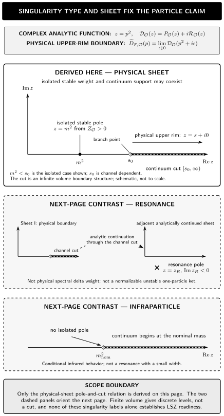
Schematic singularity map for a scalar two-point function. A positive spectral atom at produces the isolated real physical-sheet pole, while infinite-volume continuum support from produces the threshold branch point and cut. The continued-sheet resonance and infraparticle threshold are contrasts only: the former is not a physical-sheet stable pole, and the latter has no isolated mass-shell pole. The locations and shapes are not to scale, and their developed analysis is deferred.
The same distinctions are stated textually here.
| Pattern | Spectral or analytic datum | What it supports | What it does not support |
|---|---|---|---|
| Stable isolated contribution | Atom at and a real physical-sheet pole | Exact one-particle mass sector with nonzero overlap | LSZ limits or asymptotic completeness |
| Multiparticle continuum | Support from and a physical-sheet discontinuity | Threshold branch point and cut in infinite volume | A particle located at |
| Resonance contrast | Pole reached only after continuation through a channel cut | Unstable resonance diagnosis after sheet and channel are fixed | A normalizable unstable ket or physical-sheet atom |
| Infraparticle contrast | Continuous support begins at the nominal mass with no separate atom | Failure of the isolated mass-shell picture in the declared infrared setting | A decay width or second-sheet resonance |
The resonance row uses a channel-specific analytic continuation; a bump is neither necessary nor sufficient for that diagnosis Particle Data Group 2025, “Resonances,” § 50.1.1, p. 5 (PDF). The infraparticle row is a bounded signpost: under his Gauss-law hypotheses, Buchholz proves that charged states cannot be mass-operator eigenstates Buchholz 1986, pp. 331–334. It is not a universal statement about every massless theory.
A stable scalar pole plus a two-particle threshold
Section titled “A stable scalar pole plus a two-particle threshold”An exact free-field example displays both singularity types without using interaction as a diagnostic. In four spacetime dimensions, let be a canonically normalized free real scalar of mass , and define the centered operator
Normal ordering is with respect to the same free vacuum. Odd centered Gaussian correlators vanish, so the cross term between and is zero. Combining the one-particle measure of with the two-particle measure derived on the spectral-decomposition page gives
The continuum transform is logarithmically divergent before subtraction. Choose a spacelike point . A once-subtracted time-ordered function with the same pole and discontinuity is
The subtracted integrand falls as . The local constant is fixed by the extension or subtraction condition; it has zero discontinuity and changes neither the pole at nor the cut from .
Near the two-particle threshold,
so the endpoint is a square-root branch point. This example also proves that continuum support does not by itself imply interaction: the continuum belongs to a composite component of a free-field operator.
In an interacting channel the exact masses, overlaps, and density change, but the dictionary does not. A two-particle threshold is only when those particles and quantum numbers are the lightest allowed channel. A symmetry can forbid that state and move higher. Schwartz 2014, § 24.1.1, pp. 455–456; § 24.2.1, p. 469 gives a scalar example with a mass contribution and a two-particle continuum; it is an isolated stable pole only in the regime , where the decay channel is kinematically closed.
Finite volume resolves the cut into levels
Section titled “Finite volume resolves the cut into levels”A finite spatial box has discrete allowed momenta and does not retain continuous Lorentz boosts. At in an inversion-symmetric periodic box, insertion of energy eigenstates gives a schematic meromorphic sum
where and is the squared vacuum-to-level overlap with the chosen finite-volume normalization. The quadratic form combines the inversion-related positive- and negative-energy poles; without that symmetry one keeps the two linear pole sums separately.
There is no literal branch cut at finite . Only after can the multiparticle levels become dense, their weighted sum approach a continuum spectral integral, and the cut emerge. If a smearing or energy resolution is used, it is removed only after the infinite-volume limit. A level isolated at finite remains isolated only if its gap has a nonzero limit as . Bulava and Hansen 2019, § I, p. 2, Eqs. (1)–(3) (Open PDF) state the finite-volume delta-sum and the ordered limiting procedure.
The order of interpretation matters:
| Setting | Spectral pattern | Analytic pattern |
|---|---|---|
| Finite inversion-symmetric spatial volume, | Discrete energy levels | Meromorphic pole sum |
| Infinite-volume limit with a multiparticle channel | Continuous invariant-mass support | Threshold discontinuity and cut |
| Infinite volume with an isolated stable state below the channel | Delta atom plus continuum | Isolated pole plus cut |
Calling a finite sequence of levels a cut silently takes a limit that has not yet been justified.
What the dictionary does not establish
Section titled “What the dictionary does not establish”| Observation | What follows under this page’s assumptions | What still does not follow |
|---|---|---|
| with | A stable one-particle spectral sector seen by | That the particle is elementary or represented by a fundamental field |
| No pole in one chosen correlator | That operator has no nonzero isolated overlap there | That the theory contains no particle of that mass |
| A nonnegative squared overlap in the declared physical diagonal correlator | A universal probability, , or unit total weight for arbitrary | |
| A cut beginning at | Infinite-volume continuum support in that channel | A particle at the threshold, a resonance pole, or a decay width |
| An isolated physical-sheet pole | Necessary spectral input for an ordinary stable-particle route | Existence of in/out limits, infrared control, or asymptotic completeness |
Local polynomial terms and subtractions do not alter this classification. Gauge-variant correlators in an indefinite auxiliary space require a different positivity analysis, as explained on the prerequisite page.
Check your understanding
Section titled “Check your understanding”Recover the discontinuity sign. Starting from , derive and .
Check
Use . The upper-minus-lower boundary of is . Multiplying by the site’s numerator gives ; an entire polynomial contributes zero.
Classify the exact free example. Identify the stable pole, threshold, and cut for .
Check
The delta atom gives a pole at with residue in . The two-particle density begins at , so the physical cut begins there. Its square-root onset makes a branch point. The continuum is present although the underlying field theory is free.
Diagnose a finite-volume plot. A numerical spectrum at fixed shows many nearby two-particle levels above the lowest one. Is the lowest level already a branch point?
Check
No. At fixed the correlator has a discrete pole sum. A cut is an infinite-volume analytic structure obtained only when the levels become dense with the correct limiting weights.
Test operator dependence. If one operator has no pole at a known stable mass, what may be concluded?
Check
Only that this operator has zero overlap with that one-particle sector. Another operator with the same allowed quantum numbers can have nonzero overlap and display the pole.
From poles and cuts to particle limits
Section titled “From poles and cuts to particle limits”The physical-sheet result is now precise: an isolated positive spectral atom gives a real simple pole, while infinite-volume continuum support gives a discontinuity and threshold cut. Neither the threshold nor the cut is itself a particle.
Resonances, Infraparticles, and Limits of Particle Language next develops the two contrast panels in the figure. For the stable route, combine this page with Fields, Observables, and Interpolating Operators and continue to From One-Particle Poles to Scattering States. The complete reduction belongs to LSZ Reduction: Poles, Residues, and Stable External States.
The page has not analyzed general amplitudes. Landau Equations and Physical Singularities treats amplitude singularity conditions; Resonance Poles, Riemann Sheets, and Unstable States treats continued resonance sheets; and Subtracted Dispersion Relations derives amplitude dispersion constraints from their additional hypotheses.
References
Section titled “References”-
Buchholz, Detlev. “Gauss’ Law and the Infraparticle Problem.” Physics Letters B 174 (1986): 331–334. DOI.
-
Bulava, John, and Maxwell T. Hansen. “Scattering Amplitudes from Finite-Volume Spectral Functions.” Physical Review D 100 (2019): 034521. DOI. Open PDF.
-
Particle Data Group. “Resonances.” In Review of Particle Physics, 2025 review update. Official PDF.
-
Schwartz, Matthew D. Quantum Field Theory and the Standard Model. First ed. Cambridge: Cambridge University Press, 2014. DOI.
-
Weinberg, Steven. The Quantum Theory of Fields, Volume I: Foundations. First ed. Cambridge: Cambridge University Press, 1995; 2005 paperback, 2012 printing consulted. DOI.