Search Validity and Reinterpretation for Portal Models

A defensible reinterpretation is a versioned map from model parameters to the released observable and likelihood, evaluated only where both the theory description and the published response are valid. Its validity mask is fixed before fitting; correlations and dataset overlap are explicit; detector assumptions are labeled by provenance; and the conclusion is limited to the supplied model, observable, and evidence record. An exclusion contour copied from a plot, a private response model presented as official, or a post-fit EFT cut does not meet this standard.

Required background. Effective, Simplified, and Mediator Descriptions supplies the theory/width masks. Collider Measurements, Fiducial Predictions, and Likelihood Provenance supplies observable layers and released-likelihood semantics.

Helpful background. Correlated Standard Model Fits and Consistency Tests explains shared inputs, goodness of fit, and multiple-testing cautions, but its mutable fit results are not inputs here.

Reinterpretation also has a lifecycle: the durable model-to-observable contract is separate from a frozen evidence release, and corrections or supersession trigger a new bounded inference rather than silently altering the earlier result.

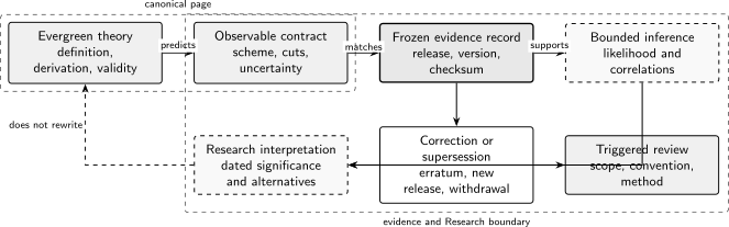
Portal limits and reinterpretations are meaningful only for an exact evidence and likelihood version. Corrections, withdrawals, and replacement releases create a new record; the schematic theory contract remains unchanged unless its assumptions change.

From model parameters to released bins

For parameters $\theta$, nuisance parameters $\eta$, and reconstructed bin $b$, a generic prediction is

$$\mu_b(\theta,\eta)=b_b(\eta) +\mathcal L_{\rm int} \int d\Phi\, R_b(\Phi;\eta) \left| \mathcal A_{\rm SM}(\Phi;\eta) +\mathcal A_{\rm BSM}(\Phi;\theta,\eta) \right|^2.$$

$R_b$ includes the released fiducial or detector response applicable to the analysis, not an assumed universal efficiency. The interference term is present automatically. A likelihood may then take a published binned form such as

$$L(\theta,\eta)= \prod_b\operatorname{Pois}\!\left(n_b\mid\mu_b(\theta,\eta)\right) \,\pi(\eta),$$

or a collaboration-released statistical model. The constraint term $\pi(\eta)$ is part of that model: its parameterization, correlations, interpolation, and auxiliary-data meaning must be preserved. Replacing it by independent Gaussian errors is a new approximation that requires validation.

The model-to-bin map has three distinct validity domains:

• Theory: gauge/anomaly consistency, perturbativity, partial-wave unitarity, mediator width, EFT truncation, and matching order.
• Response: generator phase space, fiducial definition, response/interpolation grid, object assumptions, and closure tests supplied or independently validated.
• Inference: likelihood support, nuisance priors/constraints, asymptotic calibration, dataset overlap, and coverage.

The accepted domain is their intersection. A parameter point outside one domain is not made valid by a good likelihood value.

Freeze the validity mask before fitting

Let $M_b(\theta)\in\{0,1\}$ identify bins for which the declared theory and response are usable. The rule that constructs $M_b$—including energy-transfer thresholds, maximum width, perturbativity measure, interpolation hull, and truncation tolerance—is part of the analysis specification. It is frozen, versioned, and checksummed before inspecting fitted residuals or running pseudoexperiments.

There are two legitimate responses to an invalid bin:

1. remove it through a predeclared data selection and recompute the likelihood/covariance appropriate to the reduced observable; or
2. replace the uncontrolled contribution by a documented conservative model whose nuisance treatment and coverage are validated.

Simply setting a BSM prediction to zero in an invalid region can create an artificial constraint. Changing the mask after finding the best-fit point invalidates nominal coverage because the procedure being calibrated is no longer the one used on the data.

For the mediator fixture

$$\frac{|\mathcal A_{\rm med}-\mathcal A_{\rm EFT}^{(8)}|} {|\mathcal A_{\rm med}|} =\left(\frac{E}{M}\right)^4,$$

a predeclared tolerance of $1/16$ accepts $E/M\le1/2$ away from the pole. The boundary follows from the chosen expansion and tolerance; it is not a universal EFT rule. Reproduce it by evaluating the exact residual before applying the frozen mask.

Reproducibility and provenance table

Every reinterpretation package should expose the following semantic fields. Empty fields are visible limitations, not invitations to guess.

Record field	Required content	Failure prevented
Observable identity	pole, pseudo-observable, or fiducial definition; bin edges; units; cuts; unfolding level	comparing different quantities under one label
Dataset identity	experiment/source, collision or process context, data period, dataset ID	silently mixing releases or exposures
Permanent record	publication DOI and, when applicable, exact HEPData record, table/resource DOI, explicit version, and downloaded checksum	an unversioned “latest” endpoint changing underneath the result
Statistical model	likelihood/workspace name and version, observed and auxiliary data, nuisance semantics, constraints, correlations, and morphing	reconstructing a different likelihood from a plot
Theory response	Lagrangian and parameter convention, perturbative order, matching/running, PDFs or matrix elements if used, code/environment version and checksum	ambiguous coefficient or normalization maps
Width and interference	pole convention, open channels, running/fixed-width prescription, Standard Model interference	treating an unstable mediator as an independent rate
Validity mask	event/bin variables, numerical thresholds, EFT order, perturbativity/unitarity tests, interpolation hull, mask checksum and freeze time	post-fit selection and out-of-domain extrapolation
Detector/fiducial response	official response object or clearly labeled private approximation, training/simulation domain, validation and closure	private emulation being reported as collaboration performance
Dataset dependence	event overlap, shared calibrations, common theory inputs, priors, and cross-covariance	double counting nominally separate results
Software and transformations	source commit, environment lock, random seeds, transformations, tolerances, output checksum	irreproducible numerical differences
Rights and access	license, redistribution conditions, access URL, and preserved local identity	unusable or unlawfully redistributed artifacts
Lifecycle	evidence cutoff, corrections/errata, review date, withdrawal and superseding record	a superseded result being called current

This table carries the full observable–likelihood–validity contract even when no governed figure is present. It separates a timeless method from any dated experimental application.

Exact synthetic likelihood check

Before touching external evidence, verify the inference code on a transparent Gaussian fixture:

$$y=\begin{pmatrix}1\\2\end{pmatrix}, \qquad \mu(\theta)=\begin{pmatrix}\theta\\\theta\end{pmatrix}, \qquad C=\begin{pmatrix}1&1/2\\1/2&4\end{pmatrix}.$$

Its inverse is

$$C^{-1}=\begin{pmatrix}16/15&-2/15\\-2/15&4/15\end{pmatrix}.$$

Minimizing

$$\chi^2(\theta)=(y-\mu)^{\mathsf T}C^{-1}(y-\mu)$$

gives

$$\widehat\theta =\frac{\mathbf1^{\mathsf T}C^{-1}y} {\mathbf1^{\mathsf T}C^{-1}\mathbf1} =\frac98, \qquad \chi^2_{\min}=\frac14.$$

Dropping the off-diagonal covariance changes the answer and is an intentional failure test. Independent direct inversion and Cholesky/QR evaluation should reproduce the exact result. A reproducible calculation also checks the one-dimensional interval $x\pm1$ for $x\sim N(\theta,1)$, whose exact coverage is

$$\operatorname{erf}\!\left(\frac{1}{\sqrt2}\right) =0.682689492\ldots.$$

This number validates the synthetic procedure only. It says nothing about the coverage of a non-Gaussian search with boundaries, discrete alternatives, limited simulation, or a profiled validity domain.

Correlations, combinations, and negative results

Two searches may share events, luminosity/calibration nuisances, background control regions, theory inputs, or response simulations. Combining their headline test statistics as if independent double counts information. Use a joint released likelihood or an explicitly constructed cross-covariance with a documented overlap model. If neither exists, report the missing information and keep the results separate.

For a negative result, state:

• the tested Lagrangian, parameter convention, and any fixed branching fractions;
• the observable and released likelihood/data identity;
• the prefit validity domain and excluded invalid bins/points;
• theory, response, interpolation, and statistical uncertainties;
• the test statistic and calibration or coverage study; and
• the evidence cutoff, corrections, and supersession state.

The defensible conclusion is “this released observable disfavors this valid parameter region under these assumptions,” not that the portal mechanism or every ultraviolet completion is excluded. Guidance on reusable likelihoods, cut flows, covariance, and detector-response information is provided by the LHC Reinterpretation Forum Abdallah et al. 2020, §§2–5 and the statistical-model publication recommendations of Cranmer et al. 2022, §§2–4.

Failure modes and handoffs

• A digitized contour is not a likelihood and cannot reveal nuisance correlations or coverage.
• A simplified likelihood is usable only for the information it retains; validate it against supplied benchmarks and label the approximation.
• Interpolation must remain inside a tested parameter/kinematic hull; extrapolation is a new model.
• Private simulation can support a private recast when fully documented, but it is not official detector evidence.
• Current limits, rankings, and combinations require a governed dated evidence record and remain outside this canonical method page.

For generic likelihood construction, return to Collider Measurements, Fiducial Predictions, and Likelihood Provenance. For current experimental interpretation, continue to Effective Field Theory and Tests of the Standard Model.

References

• Abdallah, Waleed, et al. “Reinterpretation of LHC Results for New Physics: Status and Recommendations after Run 2.” SciPost Physics 9 (2020): 022. DOI.
• Cranmer, Kyle, et al. “Publishing Statistical Models: Getting the Most out of Particle Physics Experiments.” SciPost Physics 12 (2022): 037. DOI.