TMD Factorization, Rapidity Evolution, and Glauber Limits

When a hard process measures a recoil $q_T\ll Q$, integrating over transverse parton momentum discards the scale that generates the large logarithms. A TMD factorization retains transverse separation, removes double-counted soft radiation, and evolves in both virtuality and rapidity. Its validity is observable- and process-specific because Wilson-line directions and Glauber exchange matter.

Required background. Collinear factorization and operator-defined PDFs supplies the integrated distributions and scheme logic. Rapidity renormalization supplies the regulator and two-scale evolution needed for lightlike sectors.

Helpful background. The eikonal approximation and Wilson lines supplies the gauge-link geometry generated by soft and collinear gluons.

The map below turns the measured scale hierarchy into a regime decision. It emphasizes that collinear, TMD, jet, and small-$x$ descriptions resolve different modes and resum different logarithms; matching them requires overlap subtraction rather than simple addition.

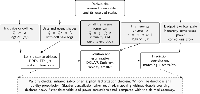
QCD factorization-regime map. The measured scales select the long-distance objects and logarithms; infrared safety or a process-specific factorization theorem, Wilson-line and rapidity conventions, Glauber cancellation, matching, and power suppression set the validity boundary. The diagram is schematic.

A low-recoil factorization statement

For production of a color-singlet system of invariant mass $Q$ in a process where TMD factorization is established, a schematic impact-parameter-space formula is

$$\frac{d\sigma}{d^2\boldsymbol q_T\,d\Phi} =H(Q,\Phi;\mu) \int\frac{d^2\boldsymbol b}{(2\pi)^2} e^{i\boldsymbol b\cdot\boldsymbol q_T} F_{a/A}(x_A,b;\mu,\zeta_A) F_{b/B}(x_B,b;\mu,\zeta_B) +Y(q_T,Q)+O\!\left(\frac{q_T^2}{Q^2}\right),$$

with $\zeta_A\zeta_B=Q^4$ in a common convention. $H$ is short-distance, the $F$ are soft-subtracted TMD distributions, and $Y$ restores the nonsingular fixed-order contribution important when $q_T$ becomes comparable to $Q$. Equivalent schemes can display an explicit soft function instead; one must not multiply subtracted TMDs by that soft factor a second time.

The formula assumes the exact angular variables, fiducial measurement, polarization, and final-state color structure used in its proof. The all-$q_T$ integral should match the corresponding collinear prediction only after the $Y$ term, perturbative orders, and convention-dependent normalizations are aligned. The original impact-parameter evolution and back-to-back factorization structure were developed by Collins and Soper 1981, §§2–7, pp. 381–443.

Why a rapidity scale appears

At fixed transverse momentum, soft and collinear modes can have the same invariant mass but very different rapidities. Dimensional regularization alone does not separate their overlap. A rapidity regulator and subtraction define finite TMD and soft objects, introducing scales conventionally denoted $\zeta$ or $\nu$ in addition to $\mu$.

In one Collins–Soper convention,

$$\frac{\partial\ln F(x,b;\mu,\zeta)} {\partial\ln\sqrt\zeta}=K(b;\mu),$$ $$\frac{d\ln F(x,b;\mu,\zeta)}{d\ln\mu} =\gamma_F\!\left(\alpha_s(\mu),\frac{\zeta}{\mu^2}\right), \qquad \frac{dK(b;\mu)}{d\ln\mu}=-\gamma_K(\alpha_s).$$

Path independence in the $(\ln\mu,\ln\sqrt\zeta)$ plane requires

$$\frac{\partial\gamma_F}{\partial\ln\sqrt\zeta}=-\gamma_K.$$

This commutativity relation is a powerful analytic and numerical check. Sign conventions for $K$ and $\gamma_K$ differ in the literature, so the three equations must be imported as a set rather than mixed across schemes. Their use in transverse-momentum resummation is developed in Collins, Soper, and Sterman 1985, §§2–4, pp. 199–224.

Natural starting scales minimize logarithms in each factor. Evolving along two different paths to common $(\mu,\zeta)$ must give the same answer to the stated logarithmic accuracy. Heavy-flavor thresholds require matching in the virtuality evolution and in the small-$b$ coefficients; a rapidity evolution kernel does not remove that requirement.

Small-b matching and the nonperturbative boundary

For $b\ll1/\Lambda_{\mathrm{QCD}}$, the TMD admits an operator expansion onto collinear PDFs,

$$F_{i/H}(x,b;\mu,\zeta) =\sum_j\left[ C_{i\leftarrow j}(b;\mu,\zeta)\otimes f_{j/H}(\mu) \right](x) +O(b^2\Lambda_{\mathrm{QCD}}^2).$$

The coefficients are perturbative and inherit the factorization and active-flavor scheme. Fourier transformation at very small $q_T$ samples large $b$, where neither this expansion nor a fixed-order kernel is perturbative. A complete prediction must then declare the nonperturbative model or fitted function, its matching prescription, and its covariance. A device such as a $b_*$ mapping is a prescription whose variation must be propagated, not a theorem.

The $q_T$ regions have distinct descriptions:

Region	Controlled structure	Required matching or input
$q_T\sim Q$	collinear fixed order	ordinary factorization and cuts
$\Lambda_{\mathrm{QCD}}\ll q_T\ll Q$	perturbative TMD evolution	$Y$ matching and common expansion
$q_T=O(\Lambda_{\mathrm{QCD}})$	TMD factorization may remain valid	nonperturbative large-$b$ input
process with color entanglement or uncancelled Glauber exchange	no generic product of two universal TMDs	a different theorem or an explicit failure statement

Wilson-line direction and Glauber limits

Initial- and final-state interactions reverse the direction of staple-shaped gauge links between Drell–Yan-type and semi-inclusive DIS definitions. Time-reversal then predicts a sign reversal for certain time-reversal-odd TMDs, while ordinary unpolarized functions have the corresponding universality relation. The process label belongs to the operator definition.

More seriously, spectator exchanges can entangle colors from different hadrons. In hadroproduction of nearly back-to-back high-transverse-momentum hadrons, explicit graphs rule out a generalized factorization into separate universal TMDs Rogers and Mulders 2010, §§II–V. This counterexample does not invalidate TMD factorization for color-singlet Drell–Yan or semi-inclusive DIS; it forbids transferring the theorem solely because the scale hierarchy looks similar.

Checks and failure modes

Two-path evolution. Evolve first in $\mu$ then $\zeta$, and in the reverse order. Their difference must be beyond the stated accuracy and numerically controlled.

Fixed-order expansion. Expand the resummed result at $q_T>0$ and compare with the singular terms of the fixed-order spectrum. The $Y$ term must remove overlap and recover the hard-recoil region.

Integrated limit. Test the $b\to0$ operator expansion and the $q_T$ integral with the same Fourier and normalization convention. A bare TMD evaluated at $b=0$ is not automatically a collinear PDF before renormalization and matching.

Regulator cancellation. The product entering the observable must be independent of the rapidity regulator through the claimed order. Residual dependence can diagnose a missing soft subtraction or mixed schemes.

Glauber statement. Name the process and measurement for which cancellation, absorption, or failure is asserted. “TMD factorization applies” without this scope is incomplete.

Common pitfalls

Setting $\mu=Q$ everywhere. That choice can minimize hard logarithms while leaving large transverse or rapidity logarithms in the TMD factors. Start each object near its natural scales and evolve.

Double counting the soft factor. Modern subtracted TMDs often already contain the required soft subtraction. Check the definition before adding a separate soft function.

Using a Gaussian as the theorem. A Gaussian transverse profile is a model for part of the large-$b$ input. The factorization theorem determines the operator and evolution structure, not that shape.

Handoff

A portable TMD prediction carries

$$\left\{\text{process and }\mathcal M,\ H,\ F^{[\text{links}]}_{i/H}, \text{soft-subtraction scheme},\ (\mu,\zeta),\ K,\gamma_F, C_{i\leftarrow j},\ Y,\ \text{large-}b\text{ input}, \text{Glauber condition}\right\}.$$

For a general treatment of the failure boundary, continue to rapidity divergences and Glauber limits. For inclusive incoming-hadron convolutions, continue to hadron-collider factorization and parton luminosities.

References

• Collins, John C., Davison E. Soper, and George Sterman. “Transverse Momentum Distribution in Drell–Yan Pair and W and Z Boson Production.” Nuclear Physics B 250, nos. 1–4 (1985): 199–224. DOI.
• Collins, John C., and Davison E. Soper. “Back-to-Back Jets in QCD.” Nuclear Physics B 193, no. 2 (1981): 381–443. DOI.
• Rogers, Ted C., and Piet J. Mulders. “No Generalized TMD-Factorization in the Hadro-Production of High Transverse Momentum Hadrons.” Physical Review D 81, no. 9 (2010): 094006. DOI. Open PDF.