

Collider Measurements, Fiducial Predictions, and Likelihood Provenance
A collider result is reusable only when the theory observable, detector response, observed and auxiliary data, likelihood or covariance, and immutable release identity form one traceable interface. A plot or unfolded central value alone is not that interface. The durable workflow is to define the fiducial measurement function, forward-fold predictions whenever possible, publish nuisance and correlation semantics, and bind every reused object to its exact version, corrections, and overlap information.
Required background. Standard Model pseudo-observables and unstable particles distinguishes pole, pseudo-observable, and fiducial layers. Validation and theory uncertainties supplies the approximation and correlation checks used below.
Helpful background. QCD prediction and uncertainty accounting supplies the scale, PDF, nonperturbative, and matching information that a collider prediction must pass forward.
The complete interface is shown below. A hard process reaches released data through event evolution, detector response, reconstruction, and fiducial selection, while pole definitions, theory uncertainties, nuisance semantics, and correlations enter the likelihood used for inference.
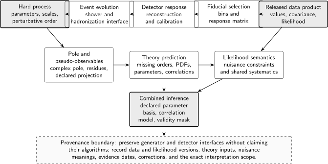
Collider inference is reproducible only when hard-process, detector, fiducial, pole, theory, data, and likelihood interfaces are versioned together. The schematic preserves these interfaces without claiming the internal algorithms of generators or detectors.
The measurement function defines the fiducial quantity
Section titled “The measurement function defines the fiducial quantity”For stable particle-level final states, a fiducial cross section can be written schematically as
where assigns an event to the accepted region or to a histogram bin. A complete specifies particle lifetimes or status convention, jet algorithm and parameters, lepton/photon dressing, isolation, overlap removal, cuts, bin edges, normalization, and units. For a fixed-order QCD prediction, infrared safety requires the relevant soft and collinear limits to leave the bin assignment unchanged,
after the unresolved momentum is mapped to the lower-multiplicity configuration. If this condition fails, real–virtual cancellation does not define the claimed perturbative observable without additional fragmentation or nonperturbative input.
Pole pseudo-observables and fiducial observables must remain distinct. A fiducial cross section uses stable final states and a measurement function. Extracting a pole mass, width, or residue from it adds a line-shape, radiation, background, interference, and acceptance model.
Forward folding and unfolding
Section titled “Forward folding and unfolding”Let label truth or fiducial bins and reconstructed categories. A prediction is connected to observed counts by
is the response, including efficiency and migration under its declared convention; is the background expectation. If each column of is a probability distribution over selected reconstructed outcomes, its sum is the efficiency and lies between zero and one. Some software absorbs luminosity or bin-width factors into the response, so dimensions and normalization must be checked rather than assumed.
Forward folding evaluates this model in reconstructed space and retains the count distribution and response nuisances. Unfolding instead constructs a derived truth-space estimate, schematically
where may depend on simulation, regularization, and a prior or reference spectrum. Its covariance is not merely the observed counting covariance transformed by a fixed inverse; response, background, and regularization choices contribute. An unfolded spectrum is valuable when these choices and the full covariance are released, but it is not automatically equivalent to the detector-level likelihood.
For any differentiable change of variables , the linear covariance rule is
The ordering, units, and evaluation point of are part of the transformation. Applying a normalized-shape transformation creates a singular covariance because the bins obey a sum constraint; one must remove a redundant coordinate or use a generalized inverse in the constrained subspace.
A released likelihood is a statistical model at fixed data
Section titled “A released likelihood is a statistical model at fixed data”Separate primary observations from auxiliary observations . A statistical model has the form
and the likelihood is this density evaluated at the observed data. A binned counting example is
The second product often appears in software as “constraint terms.” In a frequentist construction these can encode auxiliary measurements, not Bayesian priors; the release must say which. A serialized model needs the observed counts, channel/bin structure, sample yields and interpolation, parameter domains, auxiliary data, nuisance correlations, and software/schema version. Publishing only a one-dimensional profile curve can lose the nuisance response needed for combination, while multiplying models that contain the same auxiliary measurement double counts information Cranmer et al. 2022, §§2.1–2.4 and Fig. 1, pp. 4–10.
HistFactory provides one concrete channel/sample/nuisance factorization for binned models, including interpolation and auxiliary constraints Cranmer et al. 2012, §§2–4, pp. 4–21. A release that uses it still has to state the exact workspace and software version; naming the framework does not identify the model.
From collider observables to statistical inference
Section titled “From collider observables to statistical inference”| Stage | Object passed forward | Scientific check | Not claimed here |
|---|---|---|---|
| Hard process | Stable external states, perturbative order, scales, PDFs and parameter scheme | Gauge, infrared, dimension, and benchmark checks | A detector-level prediction |
| Shower and hadronization | Generator configuration, matching and nonperturbative model | Inclusive-rate preservation and matching-domain checks | First-principles detector response |
| Detector response | Calibration and migration model with nuisances | Closure and validation-domain checks | A universal response outside that domain |
| Reconstruction and selection | Dataset, object definitions, triggers, cuts, categories | Cut flow, event uniqueness, frozen selection | A pole observable without an extraction map |
| Fiducial or pole interpretation | Measurement function or pole expansion; acceptance and radiation map | Particle/reconstruction mapping and approximation tests | Model-independent extrapolation beyond the definition |
| Public release | Observed and auxiliary data; covariance or likelihood; exact identity | Reproduction of a documented benchmark | Permission to ignore correlations or corrections |
| Theory comparison | Calculation version and correlated uncertainty model | Independent benchmarks and limit checks | Validity outside the stated perturbative/EFT domain |
| Combination | Overlap rule, shared nuisances, frozen mask and test definition | Duplicate-input and covariance checks | A contemporary conclusion without dated inputs |
This table specifies interfaces, not the internal algorithms of showering, detector simulation, or reconstruction.
Provenance fields that make a result reusable
Section titled “Provenance fields that make a result reusable”Each machine-readable object should travel with a compact semantic record:
| Field | Required content | Failure detected |
|---|---|---|
| Observable definition | Particle/object convention, cuts, bin edges, normalization and units; or pole/pseudo-observable convention | Comparing different quantities with the same label |
| Dataset identity | Experiment, collision system and energy, run/sample identity, integrated exposure where applicable | Reusing overlapping events as independent data |
| Repository identity | Record and table identifiers, DOI, exact HEPData or equivalent version, stable URL | Silently following a mutable latest version |
| Integrity | File name, format/schema version, checksum when supplied or locally recorded | Byte-level substitution or corrupted transfer |
| Covariance | Bin ordering, units, component meanings, normalization constraints, parameter dependence | Permuted or dimensionally inconsistent matrices |
| Likelihood | Observed and auxiliary data, nuisance definitions/domains, correlations, interpolation, software version | Hidden priors, duplicated constraints, nonreproducible profiling |
| Theory | Calculation code/version, inputs, scales, PDFs, nonperturbative corrections, accuracy | Comparing unlike central prescriptions |
| Overlap | Shared events, controls, auxiliary data, theory inputs, and a resolution rule | Double counting across releases |
| Validity mask | Predeclared bins or parameter domain and reason | Post-fit selection of favorable inputs |
| Lifecycle | Correction notice, withdrawal or supersession relation, exact object used downstream | Replacing the historical input without disclosure |
HEPData’s record/table organization is designed to preserve numerical tables and their associated metadata, but authors and reusers still have to cite the exact record version and table rather than an unversioned landing page Maguire, Heinrich, and Watt 2017, pp. 1–6. Recommendations for reinterpretation likewise distinguish data tables, response information, simplified likelihoods, and full statistical models because they support different questions LHC Reinterpretation Forum 2020, §§2.2 and 3, pp. 8–25.
The method layer and numerical snapshot should be separate. Definitions, matrix-order rules, and reuse checks are durable. Central values, covariance files, workspace hashes, corrections, and any resulting contours are snapshot objects and must be dated and versioned together.
Independent checks and failure modes
Section titled “Independent checks and failure modes”Dimensions and bin normalization. Confirm whether each released number is a bin integral, density, normalized fraction, count, or cross section. Covariance entries carry the product of the corresponding units.
Response orientation. Inject a vector with one nonzero truth bin. The nonzero reconstructed pattern should be the documented column (or row); its sum should match the efficiency convention.
Likelihood reproduction. Evaluate the released model at a documented parameter point and reproduce its expected yields and likelihood ratio. Test nuisance values away from zero so interpolation and correlations are exercised.
Covariance geometry. Check symmetry and eigenvalues in the documented ordering. A normalized spectrum has a known null direction; an unexplained negative eigenvalue signals an invalid or mistyped matrix.
Duplicate inputs. Compare dataset identifiers, event selections, control regions, and auxiliary constraints before multiplying likelihoods. Statistical independence cannot be inferred from different paper titles.
Version mutation. Resolve every DOI or record version and calculate the expected checksum before fitting. If a correction is issued, preserve the old result’s exact input record and make a new inference with the corrected object.
Model validity. Freeze kinematic or EFT masks before examining fit residuals. A mask chosen after the outcome changes the procedure and requires its own calibration.
Common pitfalls
Section titled “Common pitfalls”Digitizing a contour and calling it a likelihood. Contours encode a chosen threshold, profiling prescription, and plotting transformation, not the underlying statistical model. Use the published likelihood or limit the claim to what the contour actually supplies.
Treating an unfolded covariance as universal. Its response, prior, and regularization can depend on the reference model. Preserve those ingredients and test forward-folded alternatives where available.
Multiplying common constraint terms. Two channels may carry the same luminosity or calibration auxiliary measurement. Correlate one shared nuisance and include the auxiliary information once.
Using an unversioned repository page. A stable landing page can point to a corrected object later. Record the exact version, table, file, and checksum used.
Informal self-check
Section titled “Informal self-check”A release provides bin values, a covariance heat map, and a one-dimensional profile-likelihood plot. Which minimum objects are still required for an exact two-parameter reuse?
Solution
At minimum, obtain machine-readable bin values and ordered covariance or, preferably, the full statistical model; exact bin definitions and units; observed and auxiliary data; nuisance meanings, domains, and correlations; the response or acceptance needed by the new prediction; dataset-overlap information; parameter validity; and exact release/version identifiers with corrections. The heat map is not a numerical covariance, and a one-dimensional profile has discarded the second parameter and generally the nuisance response.
Further study
Section titled “Further study”- Return to pseudo-observables and unstable particles when a pole or production–decay extraction is part of the published result.
- Use Higgs precision and coupling inference when response changes under coupling or tensor-structure variations.
- Use correlated Standard Model fits after identity, overlap, and nuisance semantics are complete.
- Check covariance, profiling, marginalization, and coverage on an exact synthetic fixture.
References
Section titled “References”- Cranmer, Kyle, et al. HistFactory: A Tool for Creating Statistical Models for Use with RooFit and RooStats. CERN-OPEN-2012-016 (2012). DOI · Open PDF
- Cranmer, Kyle, et al. “Publishing Statistical Models: Getting the Most out of Particle Physics Experiments.” SciPost Physics 12 (2022) 037. DOI · Open PDF
- LHC Reinterpretation Forum. “Reinterpretation of LHC Results for New Physics: Status and Recommendations after Run 2.” SciPost Physics 9 (2020) 022. DOI · Open PDF
- Maguire, Eamonn, Lukas Heinrich, and Graeme Watt. “HEPData: A Repository for High Energy Physics Data.” Journal of Physics: Conference Series 898 (2017) 102006. DOI · Open PDF