The Standard Model Lagrangian and Parameter Map

The minimal Standard Model is the most general local, Lorentz-invariant, power-counting-renormalizable theory built from its gauge fields, one Higgs doublet, and three repeated chiral matter families with no right-handed neutrinos. Its dimension-four monomials conserve baryon and lepton number classically as an accidental consequence of the field content and gauge symmetry, not as an additional defining gauge principle. Writing the theory as one object exposes missing interactions, duplicated inputs, and convention mismatches that are easy to hide when QCD, electroweak, Higgs, and flavor sectors are treated separately.

Required background. Use the field and coupling conventions of QCD in its perturbative domain and the construction of fermion masses from Yukawa couplings.

Helpful background. CKM mixing supplies the quark-flavor parameter count after the Yukawa matrices are diagonalized.

The checks that begin with the field and parameter map are summarized visually below. Read each arrow as “requires a declared interface,” not as “the upstream box proves the downstream conclusion.”

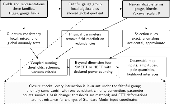
The Standard Model closes only when representation, global-form, anomaly, parameter, running, observable, and EFT checks agree. The diagram is schematic and carries no current numerical inputs.

Fields and faithful local action

For one family, the chiral fermions and Higgs transform under the Lie algebra $su(3)_C\oplus su(2)_L\oplus u(1)_Y$ as follows. The last column rewrites every fermion as a left-handed Weyl field, which is the convenient form for anomaly sums.

Physical field	$(SU(3)_C,SU(2)_L)_Y$	Left-handed anomaly field
$Q_L=(u_L,d_L)^T$	$(\mathbf3,\mathbf2)_{1/6}$	$Q$ with the same representation
$u_R$	$(\mathbf3,\mathbf1)_{2/3}$	$u^c\sim(\bar{\mathbf3},\mathbf1)_{-2/3}$
$d_R$	$(\mathbf3,\mathbf1)_{-1/3}$	$d^c\sim(\bar{\mathbf3},\mathbf1)_{1/3}$
$L_L=(\nu_L,e_L)^T$	$(\mathbf1,\mathbf2)_{-1/2}$	$L$ with the same representation
$e_R$	$(\mathbf1,\mathbf1)_{-1}$	$e^c\sim(\mathbf1,\mathbf1)_1$
$H=(H^+,H^0)^T$	$(\mathbf1,\mathbf2)_{1/2}$	complex scalar; no chiral anomaly

The charge convention is $Q=T_3+Y$ and $\widetilde H=i\sigma^2H^*$. With family indices suppressed, the gauge-invariant action can be organized without ambiguity as

$$\begin{aligned} \mathcal L_{\mathrm{SM}}={}& -\frac14G^a_{\mu\nu}G^{a\mu\nu} -\frac14W^I_{\mu\nu}W^{I\mu\nu} -\frac14B_{\mu\nu}B^{\mu\nu} \\ &+\sum_{\psi=Q_L,u_R,d_R,L_L,e_R}\bar\psi\,iD\!\!\!/\,\psi +(D_\mu H)^\dagger D^\mu H -V(H) \\ &-\left(\bar Q_LY_dHd_R+\bar Q_LY_u\widetilde H u_R +\bar L_LY_eHe_R+\text{h.c.}\right) \\ &+\frac{\theta_3g_s^2}{32\pi^2}G^a_{\mu\nu}\widetilde G^{a\mu\nu} +\mathcal L_{\mathrm{gf}}+\mathcal L_{\mathrm{gh}}, \end{aligned}$$

where

$$D_\mu=\partial_\mu-ig_sG_\mu^aT^a-igW_\mu^I t^I-ig'YB_\mu, \qquad V(H)=-m^2H^\dagger H+\lambda(H^\dagger H)^2.$$

Each representation in the table makes every displayed monomial neutral. For example, $Y(\bar Q_L)+Y(\widetilde H)+Y(u_R)=-1/6-1/2+2/3=0$. This one-line check detects the common error of using $H$ rather than $\widetilde H$ in the up-type term. The sector decomposition and representations agree with the explicit Standard Model constructions in Schwartz 2014, §§29.1–29.3, pp. 584–602 and Weinberg 1996, ch. 21.

$\mathcal L_{\mathrm{gf}}+\mathcal L_{\mathrm{gh}}$ is required to define perturbation theory but is not a new physical sector. Its parameters must disappear from pole positions and on-shell or fiducial observables after a consistent finite-order calculation. Likewise, the topological term is a total derivative in perturbation theory but its coefficient is a genuine nonperturbative parameter once the global and boundary conditions admit nontrivial sectors Schwartz 2014, §30.5.2, pp. 636–637.

From matrices to independent parameters

Before field redefinitions, the three complex $3\times3$ Yukawa matrices contain many redundant coordinates. With no neutrino-mass operator, unitary flavor rotations reduce them to nine charged-fermion masses, three CKM angles, and one CKM phase. A useful map is:

Sector	Convenient renormalized coordinates	Independent physical content in the minimal model	Typical dependent outputs
Gauge	$g_s,g,g'$ in a stated scheme and at a stated scale	three gauge couplings	$e$, $\sin\theta_W$, running masses and vertices
Higgs potential	$m^2,\lambda$ before symmetry breaking	two scalar-sector parameters	$v$, the Higgs pole mass after radiative matching
Quark Yukawa	$Y_u,Y_d$ modulo flavor rotations	six masses, three angles, one CP phase	CKM elements and Yukawa eigenvalues
Charged-lepton Yukawa	$Y_e$ modulo flavor rotations	three masses	charged-lepton Yukawa eigenvalues
Strong topology	$\theta_3$ together with Yukawa phases	one invariant $\bar\theta$	CP-odd hadronic observables

Thus the minimal renormalizable model with exactly massless neutrinos has nineteen independent continuous parameters: three gauge couplings, two Higgs-potential parameters, nine charged-fermion masses, four CKM parameters, and $\bar\theta$. This is the sum of the independent entries in the preceding table; the flavor reduction and invariant strong phase are treated in Schwartz 2014, §§29.1–29.3 and 30.5.2, pp. 584–602 and 636–637. This count is a statement about a particular field content and quotient by allowed field redefinitions—not about which measured quantities are used as inputs. Adding neutrino masses, right-handed neutrinos, or higher-dimensional operators changes the count and must be declared rather than silently folded into “the Standard Model.”

An electroweak input scheme trades coordinates, for example $(g,g',v)$ for three precisely defined observables. Such a trade is invertible only at a fixed perturbative order and with mass, tadpole, width, and subtraction prescriptions stated. The electroweak input-scheme page develops that translation; the invariant check is that a physical observable agrees after converting all inputs and counterterms to the same order.

A term-by-term assembly test

Given a proposed Standard Model Lagrangian, the following sequence finds most structural errors before any long calculation.

1. Representations: apply $Q=T_3+Y$ to every component and verify that color and weak multiplicities are explicit.
2. Gauge invariance: sum hypercharges and contract every $SU(2)$ and $SU(3)$ index in each interaction.
3. Hermiticity: include the conjugate of every non-Hermitian Yukawa term and use real coefficients for Hermitian operators.
4. Power counting: in four dimensions, retain operators of canonical dimension at most four for the renormalizable action.
5. Redundancies: quotient by unitary field redefinitions before counting phases and mixing angles.
6. Quantum consistency: run the local and global anomaly checks; classical gauge invariance alone is insufficient Weinberg 1996, ch. 22.
7. Input semantics: label the renormalization scheme, scale, threshold content, mass definition, and electroweak input set.

As a representative round trip, diagonalize

$$Y_u=U_{uL}y_uU_{uR}^\dagger, \qquad Y_d=U_{dL}y_dU_{dR}^\dagger, \qquad V_{\mathrm{CKM}}=U_{uL}^\dagger U_{dL}.$$

Returning to the original weak basis by the inverse rotations reconstructs both matrices, while masses and rephasing-invariant combinations such as the Jarlskog invariant remain unchanged. Failure of that round trip means a phase, rotation, or normalization has been double counted.

What this action does not settle

The local Lagrangian does not by itself select a unique global quotient of $SU(3)\times SU(2)\times U(1)$, prove anomaly cancellation, decide the ultraviolet fate of the Higgs potential, or justify a particular EFT truncation. Those are distinct questions because they probe, respectively, genuine line and bundle data, the quantum measure, scale evolution and tunneling, and a declared expansion beyond dimension four.

The typed output of this page is

$$\left\{ G_{\mathrm{gauge}},\ \{R_i,Y_i\},\ g_s,g,g',m^2,\lambda,Y_u,Y_d,Y_e,\bar\theta;\ \text{scheme},\mu,\text{thresholds},\text{input set} \right\}.$$

Feed it next into the global-form test, the anomaly sums, or the SMEFT/HEFT observable map, depending on whether the question concerns faithful gauge action, quantum consistency, or controlled deformations.

References

• Schwartz, Matthew D. Quantum Field Theory and the Standard Model. Cambridge University Press, 2014, §§29.1–29.3 and 30.5.2, pp. 584–602 and 636–637. DOI.
• Weinberg, Steven. The Quantum Theory of Fields. Vol. II: Modern Applications. Cambridge University Press, 1996, chs. 21–22. DOI.