

Lattice Regulators and Target Continuum Theories
A spacetime lattice defines a finite regulated model; it represents a target continuum QFT only when the fields, measure, geometry, bare parameters, observables, tuning conditions, symmetry-restoration tests, and ordered limits are specified together. The decisive object is therefore not “the lattice action” alone. It is a family of regulated theories and renormalized observables, indexed by cutoff and volume, whose convergence is tested along a declared trajectory.
Required background. Regulators, Cutoffs, and Continuum Limits supplies the distinction between a regulated object and regulator removal.
Helpful background. Regulated Bosonic Field Integrals explains how a finite-dimensional measure replaces a formal bosonic functional measure. QFT Regulator Families and Their Tradeoffs places the lattice among other regulators.
The lattice regulator as complete scientific data
Section titled “The lattice regulator as complete scientific data”Target and regulator card. Work at finite spacings and extents on a declared Euclidean cell complex. The field domains, measure, boundary conditions, constraints, bare action, and regulator-level observable are local data; none is inferred from the word “lattice.” The scalar benchmark below uses real site fields and periodic hypercubic geometry, while the continuum statement always names the tuned trajectory and order of limits.
Consider a Euclidean theory in dimensions. A hypercubic realization has sites
but these symbols do not yet define the theory. One must also state whether opposite faces are identified, twisted, or left open; which variables live on sites, links, or higher cells; the integration or summation measure; and any constraints. The regulated expectation value is then an ordinary finite-dimensional expression,
Here includes the domain and constraints, includes all Jacobians, denotes bare parameters, and is a regulator-level operator. The page uses the site-wide Euclidean and natural-unit conventions; the lattice spacings, boundary conditions, field normalization, and measure are local choices.
The following record is the minimum needed to interpret a result. It also realizes the chapter’s target–regulator–limit comparison table.
| Part of the specification | What must be stated | Free-scalar example |
|---|---|---|
| Target theory | Dimension, continuum fields, interactions, state, and renormalized observable | Massive real scalar in Euclidean dimensions; two-point function at nonzero separation |
| Regulated variables | Location, domain, normalization, constraints, and measure | on sites; |
| Geometry | Lattice, , , , orientation, boundaries | Isotropic ; periodic box |
| Bare definition | Action and all bare parameters | Nearest-neighbor action with and, if interacting, |
| Exact finite- structure | Exact symmetries and identities | Translations by lattice vectors, hypercubic rotations, |
| Broken target structure | Symmetries or relations not exact at finite cutoff | Continuous translations and rotations |
| Tuning conditions | Independent renormalized quantities held fixed | Fixed pole mass (or in a declared finite-volume scheme); for the free target |
| Observable map | Renormalization, mixing, subtraction, scale | away from contact |
| Scale hierarchy | Dimensionless cutoff, volume, and physical ratios | , , and separations |
| Limit order | Limits, held-fixed quantities, convergence norm or observable | at fixed physical , followed by |
| Convention translation | Field, Fourier, source, orientation, and normalization conventions, with a named source of truth | Translate the discrete Fourier pair and verify the Kronecker delta and propagator normalization |
| Independent tests | Analytic anchor and structurally distinct checks | Free dispersion, directional correlators, transfer positivity, alternative action |
The finite lattice is exact within this specification. That exactness does not propagate automatically to the continuum interpretation.
From one model to a convergent family
Section titled “From one model to a convergent family”Let label a sequence. A target claim requires bare parameters , volumes , and lattice operators chosen by renormalized conditions. For a dimensionless target observable , a schematic asymptotic ansatz has the form
The exponent , the finite-volume function , mixed cutoff–volume terms, logarithms, and the omitted terms depend on the action, operator, state, and symmetries. Writing such an expansion is a hypothesis to be tested, not permission to fit any few points to a smooth curve. Symanzik’s effective-action analysis explains why local lattice artifacts often organize into powers of after lower-dimensional operators have been tuned, but the permitted powers and logarithms are formulation dependent Symanzik 1983, Part I, pp. 187–204 and Part II, pp. 205–227.
The formulation map below shows the logic to inspect: every declared route begins with a finite regulator and reaches a continuum statement only after resolving its observable map, independently varied error directions, an independent validation test, and explicit limits. A step that is genuinely irrelevant to a formulation is marked not applicable rather than silently skipped.
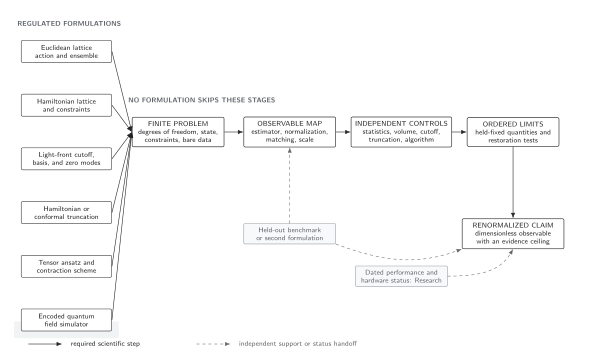
Regulated formulations provide different finite problems, but every claimed route must resolve—or explicitly mark inapplicable—the observable definition, error controls, independent validation, and ordered limits. The endpoint is a dimensionless renormalized comparison, using a declared reference scale when the original observable has units, with explicit supporting results and limitations. The diagram is schematic and not to scale.
The arrows in that figure are logical requirements, not claims that all limits commute. The separate limit-order diagram below makes this warning concrete.
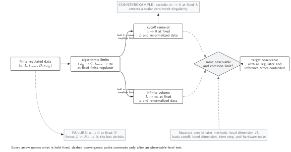
Both main routes apply cutoff removal and infinite volume while matching the target data before their results are compared. A broken phase and the periodic massless scalar give genuine order tests; at fixed site count is instead a misidentified path because the box shrinks. Other truncation and time-evolution axes need their own declared schedules. Schematic, not to scale.
A fully checkable periodic scalar
Section titled “A fully checkable periodic scalar”For an isotropic periodic lattice, take
With the normalized transform
the action diagonalizes:
Therefore
This finite-regulator identity provides three independent checks.
First, dimensional analysis gives and . Second, positivity follows for because every eigenvalue of the kernel is positive. Third, at fixed physical momentum,
so the propagator approaches the continuum free propagator with a leading directional artifact. This is an analytic benchmark for code and for later interacting calculations. It does not establish an interacting continuum limit.
The massless periodic case is an adversarial check. At , the eigenvalue vanishes and the Gaussian integral over the constant mode diverges. Removing that mode by hand defines a different measure; it must be stated and justified. A reported propagator that silently omits it has not implemented the declared theory.
What can be exact, approximate, and inferred
Section titled “What can be exact, approximate, and inferred”It is useful to label each step by logical status:
- The finite sum or integral and its algebraic symmetries can be exact.
- Monte Carlo evaluation of it is statistical and algorithm dependent.
- Operator matching and cutoff expansions are approximate unless established nonperturbatively.
- A continuum extrapolation is an inference conditioned on the tuned trajectory and fit model.
- Universality is a statement that matched trajectories in the same fixed-point basin share a continuum limit; visual similarity at one spacing is not such evidence.
Wilson’s formulation of lattice gauge theory made the regulator’s exact local gauge symmetry and nonperturbative strong-coupling expansion central Wilson 1974, §§2–4. The modern lesson is broader: preserve exact structure where possible, list what the regulator breaks, and test restoration using renormalized observables. General renormalization-group explanations of why distinct microscopic actions can share a continuum fixed point remain the responsibility of Relevant, Marginal, and Irrelevant Directions.
Failure modes and stop conditions
Section titled “Failure modes and stop conditions”A named action without a target. “Wilson action,” “nearest-neighbor scalar,” or “quantum link model” specifies only part of the finite problem. Stop until the target theory, observable, tuning, and limits are named.
One sequence changes several physical scales. If is fixed while , then . This is not the continuum limit at fixed physical volume and certainly not the infinite-volume limit.
A bare observable is treated as physical. Even if converges numerically, the operator may mix, require additive subtraction, or carry a multiplicative normalization. The observable map must be specified before extrapolation.
One regulator is taken as proof of universality. Internal convergence along one action family tests that family. A second discretization with the same target field content and symmetries but different leading artifacts is stronger evidence after relevant data are matched; it is still a cross-check, not a proof that either continuum limit exists.
Limits are exchanged by notation. Writing , , and on one line does not prove commutation. Test the two iterated limits on the same observable or state a theorem that applies.
Observable-level validation checklist
Section titled “Observable-level validation checklist”Before accepting a lattice-to-continuum statement, verify that:
- the target observable is dimensionless or is quoted in a declared scale-setting convention;
- the action, measure, boundary data, and exact constraints reproduce an analytic finite-regulator case;
- each lattice spacing has sufficiently separated volume and cutoff scales;
- the bare trajectory is fixed by independent renormalized conditions;
- operator matching and mixing use a named scheme and scale;
- cutoff, volume, statistics, fit, and algorithmic errors are varied independently;
- at least one symmetry-restoration or Ward-identity test is withheld from the tuning conditions; and
- an alternative action, observable definition, formulation, or controlled theorem supports the same target after matching.
A numerical continuation of this benchmark must reproduce the analytic result above and retain the full regulator specification.
Exercises
Section titled “Exercises”1. A shrinking-box counterexample. Let and . Find and the smallest nonzero periodic momentum. Explain why neither remains fixed in physical units.
Solution
shrinks to zero, while diverges. Although the ultraviolet cutoff grows, the sequence removes the low-momentum physics one intended to keep. A fixed-volume sequence requires .
2. Independent cutoff and volume changes. For a massive free scalar, propose three ensembles that vary while holding fixed and three that vary while holding fixed. State how the bare mass is tuned.
Solution
Choose, for example, fixed with and set on every ensemble. For a volume study choose fixed with , giving . Holding one dimensionless control fixed lets the two error directions be probed separately; three points do not by themselves establish the assumed cutoff or volume dependence.
What you can now do
Section titled “What you can now do”You should now be able to write a complete finite-lattice specification and distinguish an exact regulator-level calculation from a continuum-QFT claim. You should also be able to reject a proposed extrapolation when its observable map, tuning trajectory, restoration test, or limit order is missing. Continue with Lattice Geometry, Boundaries, and Anisotropy to turn the abstract geometry fields in the specification into momenta, images, edge terms, and scale hierarchies.
References
Section titled “References”- Symanzik, Kurt. “Continuum Limit and Improved Action in Lattice Theories. I. Principles and Theory.” Nuclear Physics B 226, no. 1 (1983): 187–204. doi:10.1016/0550-3213(83)90468-6.
- Symanzik, Kurt. “Continuum Limit and Improved Action in Lattice Theories. II. O() Nonlinear Sigma Model in Perturbation Theory.” Nuclear Physics B 226, no. 1 (1983): 205–227. doi:10.1016/0550-3213(83)90469-8.
- Wilson, Kenneth G. “Confinement of Quarks.” Physical Review D 10, no. 8 (1974): 2445–2459. doi:10.1103/PhysRevD.10.2445.
Further reading
Section titled “Further reading”- DeGrand, Thomas, and Carleton DeTar. Lattice Methods for Quantum Chromodynamics. World Scientific, 2006. doi:10.1142/6065.
- Montvay, István, and Gernot Münster. Quantum Fields on a Lattice. Cambridge Monographs on Mathematical Physics. Cambridge University Press, 1994, chs. 1–2. doi:10.1017/CBO9780511470783.