LSZ Reduction: Poles, Residues, and Stable External States

LSZ turns a time-ordered correlator into a scattering amplitude when each external channel contains an isolated simple pole at the real mass of a stable particle, with nonzero positive residue, and when wave-packet in/out states exist. Multiplying by the inverse pole, dividing by the square root of its residue, taking every external momentum on shell, and retaining the connected part leaves the convention-normalized S-matrix amplitude.

Required background. S-Matrix and T-Matrix Normalization fixes $\mathcal M$ and the overall delta function. From One-Particle Poles to the Scattering Handoff supplies the readiness test: a field must overlap a stable, isolated one-particle sector.

Helpful background. The Källén–Lehmann Representation explains the spectral origin of poles and continua. Lorentzian Boundary Conditions and the $i\epsilon$ Prescription distinguishes the Feynman boundary value used in the correlator.

The external pole and its residue

Let $\phi$ be a Hermitian scalar interpolating field and $|\mathbf p\rangle$ a stable one-particle state of physical mass $m$, normalized by

$$\langle\mathbf p'|\mathbf p\rangle =(2\pi)^3 2E_{\mathbf p}\delta^{(3)}(\mathbf p'-\mathbf p).$$

Choose the field phase so that

$$\langle\Omega|\phi(0)|\mathbf p\rangle=\sqrt Z, \qquad Z>0.$$

Near the isolated pole, the exact time-ordered two-point function is

$$\widetilde G_2(p) =\frac{iZ}{p^2-m^2+i0} +\text{terms less singular at }p^2=m^2.$$

The pole location is the physical mass; $Z$ measures the overlap of this particular field with the normalized particle. Rescaling $\phi$ changes $Z$ but cannot change an S-matrix element, because LSZ contributes one factor $Z^{-1/2}$ for each external leg. A composite interpolating operator works equally well if it has the same nonzero one-particle overlap. Weinberg’s pole-factorization argument and arbitrary-spin extension are given in Weinberg 1995, §§ 10.2–10.3, pp. 430–441.

Wave packets turn the asymptotic condition into a boundary term

For a positive-frequency Klein–Gordon solution

$$f_t(\mathbf x) =\int\frac{\mathrm d^3\mathbf p}{(2\pi)^3 2E_{\mathbf p}} f(\mathbf p)e^{-ip\cdot x},$$

the Klein–Gordon inner product isolates a creation or annihilation operator. Applied to the interacting field, the asymptotic condition is schematically

$$a_{\mathrm{in/out}}(f) =\frac{i}{\sqrt Z} \lim_{t\to\mp\infty} \int\mathrm d^3\mathbf x\, f_t^*(\mathbf x) \overleftrightarrow{\partial_0}\phi(t,\mathbf x),$$

with the upper time limit chosen for out and the lower for in. The equality is a limit on packets, not sharp plane waves.

Integrating $(\Box+m^2)$ over spacetime converts the bulk integral to the difference between these temporal boundaries. Inside a time-ordered product, repeating this step for every external packet replaces asymptotic creation and annihilation operators by Klein–Gordon operators acting on the correlator. Schwartz carries out this boundary-term derivation in Schwartz 2014, § 6.1, pp. 70–74, while the original field-to-S-matrix formulation is due to Lehmann, Symanzik, and Zimmermann 1955, pp. 205–225.

The underlying Green identity is visible on any time slab $[t_-,t_+]$. Because $(\Box+m^2)f=0$,

$$\int_{t_-}^{t_+}\mathrm d^4x\, f^*(x)(\Box+m^2)\phi(x) =\left. \int\mathrm d^3\mathbf x\, f^*(x)\overleftrightarrow{\partial_0}\phi(x) \right|_{t_-}^{t_+},$$

up to spatial boundary terms suppressed by the packet. The LSZ operator is therefore not guessed from a drawn propagator: it is the bulk operator whose integral measures the difference between the out and in boundary annihilators.

The scalar reduction formula

Let $p_1,\ldots,p_n$ be incoming and $p'_1,\ldots,p'_m$ outgoing stable scalar momenta. With all external momenta on their positive-energy mass shells, the connected formula in the site convention is

$$\begin{aligned} &\langle p'_1\cdots p'_m,\mathrm{out} |p_1\cdots p_n,\mathrm{in}\rangle_c\\ &=\left[\prod_{a=1}^{m} \frac{i}{\sqrt Z}\int\mathrm d^4x_a\, e^{+ip'_a\cdot x_a}(\Box_{x_a}+m^2)\right]\\ &\quad\times \left[\prod_{b=1}^{n} \frac{i}{\sqrt Z}\int\mathrm d^4y_b\, e^{-ip_b\cdot y_b}(\Box_{y_b}+m^2)\right]\\ &\quad\times \langle\Omega|\mathrm T\{ \phi(x_1)\cdots\phi(x_m) \phi(y_1)\cdots\phi(y_n)\}|\Omega\rangle_c. \end{aligned}$$

For different species, use its own $m_r$, $Z_r$, and interpolating field on each leg. The phases distinguish outgoing from incoming states. Contact terms generated when derivatives meet time ordering do not create the simultaneous set of external one-particle poles and therefore vanish under the complete on-shell residue extraction.

In momentum space, the same statement is especially transparent. Near all external poles, a connected Green function factorizes as

$$\widetilde G_c \sim \left[\prod_{a=1}^m \frac{i\sqrt{Z_a}}{p_a'^2-m_a^2+i0}\right] i(2\pi)^4\delta^{(4)}(P_f-P_i)\mathcal M_{fi} \left[\prod_{b=1}^n \frac{i\sqrt{Z_b}}{p_b^2-m_b^2+i0}\right].$$

LSZ multiplies by $(p^2-m^2)/(i\sqrt Z)$ on every leg and takes the on-shell limits. This is amputation plus residue normalization, not merely deleting drawn propagator lines. Srednicki derives the formula and the field-overlap condition in Srednicki 2007, § 5, pp. 49–56.

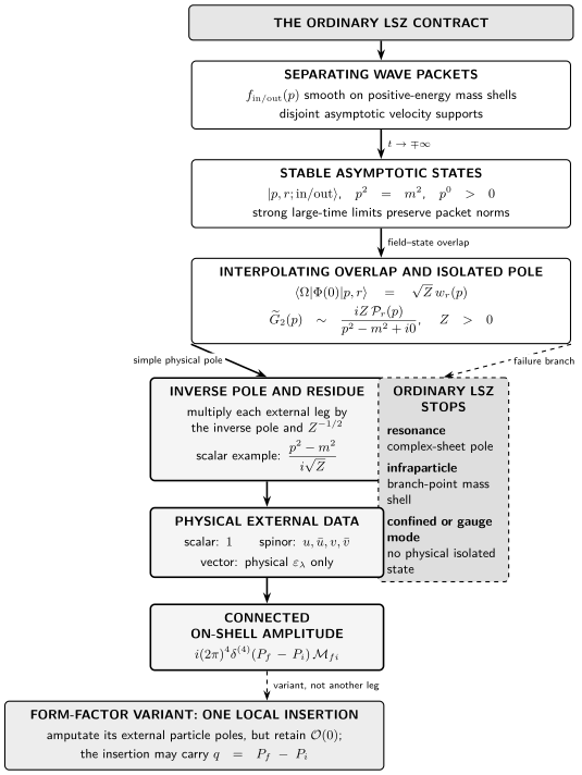
The figure summarizes the successful path and its stopping points. Follow the solid central route; the dashed branch lists spectral situations for which the scalar inverse-pole operation has no ordinary external-state meaning.

The ordinary LSZ contract. Separating wave packets and an isolated real pole $iZ/(p^2-m^2+i0)$ define stable external states; every external leg is multiplied by its inverse pole and $Z^{-1/2}$ before the on-shell limit. Spinors and physical polarizations replace the scalar endpoint for spinning states, while a declared local operator insertion remains unamputated. The diagram is schematic and not to scale.

Figure stage	Mathematical operation	Check
packet	take the strong in/out limit on smooth momentum support	packet norms are preserved
pole	isolate a simple real pole and its positive residue	the same $m$ appears in the state and propagator
amputation	multiply by $(p^2-m^2)/(i\sqrt Z)$ per scalar leg	a free external propagator leaves unit residue
on-shell limit	set $p^0=+\sqrt{\mathbf p^2+m^2}$ after multiplication	the result is finite and carries one overall delta function
failure branch	find no isolated physical pole or no asymptotic state	ordinary LSZ is not asserted

A four-point normalization check

For $\mathcal L_{\mathrm{int}}=-\lambda\phi^4/4!$ and a field normalized with residue $Z=1$ at tree level, the connected four-point function has the pole part

$$\widetilde G_c^{(4)} =\left[\prod_{j=1}^{4}\frac{i}{p_j^2-m^2+i0}\right] (-i\lambda)(2\pi)^4\delta^{(4)}\!\left(\sum_j p_j\right),$$

where the displayed momenta are taken incoming for this equation. Multiplying by $(p_j^2-m^2)/i$ on all four legs leaves $-i\lambda$. Since $i\mathcal M=-i\lambda$, the result is $\mathcal M=-\lambda$, matching the direct S-matrix convention check.

The same calculation shows why a missing $Z^{-1/2}$ is physical. The exact two-point function has pole residue $iZ$, whereas factorization of a multipoint correlator supplies one overlap $\sqrt Z$ on each external leg. The four-point correlator therefore contains $(\sqrt Z)^4$ from its external overlaps, and four LSZ factors cancel them exactly.

The hypotheses, stated without shorthand

Ordinary reduction requires:

• a vacuum representation with suitable translation and Lorentz symmetry;
• stable positive-norm one-particle states of physical masses $m_r$;
• isolated simple poles separated sufficiently from multiparticle spectral support;
• interpolating fields or operators with finite nonzero overlaps $\sqrt{Z_r}$;
• in/out wave operators for the packet configurations being scattered;
• adiabatic and large-time limits that do not leave uncanceled long-range interactions;
• a time-ordered Lorentzian correlator with the Feynman $+i0$ boundary value; and
• connected reduction, with identity and spectator pieces handled separately.

These are physical assumptions, not consequences of perturbative notation. The rigorous existence and distributional hypotheses are developed in LSZ Reduction and Amputated Distributions.

Where ordinary LSZ does not apply

Unstable particles. A resonance is associated with a pole reached by analytic continuation to an unphysical sheet, generally at complex invariant mass. It is not a normalizable asymptotic ket, so it belongs inside amplitudes or controlled resonance approximations, not as an exact LSZ external leg.

Infraparticles. With unscreened massless radiation, a charged field can have a branch point rather than an isolated mass pole. A simple scalar analogue in which a pole merges with continuum support shows the same residue obstruction: a finite on-shell $Z$ cannot then be imposed Srednicki 2007, § 27, pp. 172–174.

Confined colored fields. A gauge-fixed quark or gluon propagator is not evidence for a physical colored asymptotic state. External states must belong to the physical spectrum.

Nonstationary backgrounds. If no common past and future particle notion exists, an in-out S-matrix may not be the appropriate observable. In-in expectation values or curved-spacetime Bogoliubov data answer different questions.

Common pitfalls

“LSZ says every propagator pole is a particle.” The pole must belong to a physical positive-norm stable state and be isolated on the real mass shell. Gauge artifacts and resonance poles fail this test.

“Amputation means erase the external propagators in a diagram.” The exact operation is a residue limit on the full connected correlator. Diagram deletion is a perturbative shorthand after normalization has been fixed.

“Set $p^2=m^2$ before multiplying.” That produces zero times infinity. Multiply by the inverse pole first, then take the on-shell limit.

“Field-strength renormalization changes the S-matrix.” A field rescaling changes $Z$ and the correlator residues inversely. The LSZ-normalized amplitude is unchanged.

Check your understanding

1. If $\phi'=c\phi$, how do the two-point residue and an $N$-point correlator change, and why is $\mathcal M$ invariant?

   Answer

   The residue becomes $Z'=|c|^2Z$, while the correlator acquires one factor $c$ for every occurrence of the field. Each LSZ factor contributes $(Z')^{-1/2}$, canceling the rescaling on its external insertion, so the final amplitude is unchanged up to the consistently chosen particle-state phases.

2. A propagator behaves as $(p^2-m^2+i0)^{-1+\alpha}$ with nonzero $\alpha$. What part of the reduction fails?

   Answer

   There is no isolated simple pole with finite nonzero residue. Multiplication by $p^2-m^2$ does not leave a finite constant, so the field does not support an ordinary LSZ external leg under these assumptions.

3. Why may contact terms from differentiating time ordering be omitted only after the complete external residue is specified?

   Answer

   A contact term can be nonzero and is essential to distributional identities such as $(\Box+m^2)D_F=-i\delta$. What it lacks in the ordinary scalar reduction is the simultaneous product of isolated one-particle poles for every external channel. Multiplying by all inverse poles and taking the joint on-shell residue removes such a term. Dropping it before identifying that joint singularity would be unjustified, especially for derivative interactions or retained operator insertions.

Continue

LSZ for Spinor and Vector External States replaces scalar residues by spin projectors and physical polarizations. Cross Sections and Decay Rates uses the stripped $\mathcal M$. For failure modes, continue to Resonance Poles, Riemann Sheets, and Unstable States or Dressed States and Infrared-Finite Scattering.

References

• Lehmann, Harry, Kurt Symanzik, and Wolfhart Zimmermann. “Zur Formulierung quantisierter Feldtheorien.” Il Nuovo Cimento 1, no. 1 (1955): 205–225. DOI.
• Schwartz, Matthew D. Quantum Field Theory and the Standard Model. Cambridge: Cambridge University Press, 2014. DOI.
• Srednicki, Mark. Quantum Field Theory. Cambridge: Cambridge University Press, 2007. DOI.
• Weinberg, Steven. The Quantum Theory of Fields. Volume I: Foundations. Cambridge: Cambridge University Press, 1995. DOI.