Rapidity Renormalization and Two-Scale Evolution

Dimensional regularization separates modes with different invariant masses, but it cannot distinguish modes that have the same virtuality and are separated only by a large boost. Their separate soft and collinear matrix elements can therefore contain divergent integrals over rapidity even though the complete amplitude is finite. A rapidity regulator converts those divergences into counterterms and introduces a scale $\nu$ whose evolution resums logarithms of rapidity ratios.

This page derives the rapidity counterterms of a one-loop massive Sudakov form factor in the $\eta$ regulator, obtains the coupled $\mu$ and $\nu$ anomalous dimensions, and verifies path independence explicitly. The regulator and individual sector functions are scheme dependent; cancellation in the sector sum and the integrability of two-scale evolution are the physical tests.

Required background. Matching onto Factorized Operator Structures supplies the soft and collinear sectors and their overlap subtractions. Evolution Kernels, Consistency Relations, and Resummation Architecture supplies the single-scale kernel logic. Rapidity Divergences, Glauber Exchange, and Factorization Limits explains why rapidity consistency does not by itself prove cancellation of Glauber exchange.

Equal virtuality, unequal rapidity

Choose null vectors $n^2=\bar n^2=0$ with $n\!\cdot\!\bar n=2$, and write momentum components in the order $(n\!\cdot p,\bar n\!\cdot p,p_\perp)$. For a hard scale $Q$, an infrared mass $M$, and $\lambda=M/Q\ll1$, the relevant scalings are

$$\begin{aligned} p_n&\sim Q(\lambda^2,1,\lambda), &p_n^2&\sim M^2, \\ p_{\bar n}&\sim Q(1,\lambda^2,\lambda), &p_{\bar n}^2&\sim M^2, \\ p_s&\sim Q(\lambda,\lambda,\lambda), &p_s^2&\sim M^2. \end{aligned}$$

All three modes have the same virtuality. Their rapidities,

$$y(p)=\frac12\ln\left|\frac{\bar n\!\cdot p}{n\!\cdot p}\right|,$$

are instead centered near $+\ln(1/\lambda)$, $-\ln(1/\lambda)$, and $0$. On a fixed-invariant-mass hyperbola one may set $k^+=\kappa e^y$ and $k^-=\kappa e^{-y}$. Dimensional regularization controls the transverse and invariant-mass integrations but leaves

$$\int_0^\infty\frac{dk^+}{k^+}=\int_{-\infty}^{\infty}dy$$

unregulated. The endpoints are the soft–collinear overlap viewed as an infinite boost, not an additional ultraviolet limit in $k^2$.

Divergence	Direction in loop momentum	Regulator and scale	Renormalized evolution
Ultraviolet	Increasing invariant mass or transverse momentum	$d=4-2\epsilon$ and $\mu$	$\mu\,d/d\mu$
Rapidity	Increasing boost at fixed invariant mass	$\eta$ and $\nu$ in the scheme below	$\nu\,d/d\nu$

Mixed poles such as $1/(\eta\epsilon)$ are expected: a rapidity counterterm can itself have ultraviolet scale dependence. They do not identify the two divergences.

The η regulator and the one-loop overlap

Consider the spacelike color-singlet quark current in a gauge theory whose gauge boson has mass $M$, used here as an infrared regulator. Work in Feynman gauge and subtract both $\epsilon$ and $\eta$ poles minimally. For an emission of momentum $k$, the $\eta$ prescription modifies collinear and soft Wilson-line vertices schematically as

$$\frac{\bar n^\mu}{\bar n\!\cdot k} \longrightarrow \frac{\bar n^\mu}{\bar n\!\cdot k}\, w^2\left(\frac{\nu}{|\bar n\!\cdot k|}\right)^\eta,$$

and

$$\frac{n^\mu}{n\!\cdot k} \longrightarrow \frac{n^\mu}{n\!\cdot k}\, w\left(\frac{\nu}{|2k^3|}\right)^{\eta/2}.$$

The auxiliary $w$ keeps track of rapidity renormalization and is set to one after differentiation. The relative power of $\eta$ follows from the soft line having two eikonal attachments where the corresponding collinear graph has one. The order of limits is part of the scheme:

$$\eta\to0\quad\text{before}\quad\epsilon\to0, \qquad \frac{\eta}{\epsilon^m}\to0\quad(m>0).$$

Taking the limits in the opposite order leaves the fixed-virtuality hyperbola before removing the rapidity cutoff and mixes the intended sector boundaries.

The leading-power current factorizes as

$$J^\mu =H(Q^2,\mu)\, J_n(M;\mu,\nu/Q)\, \gamma_\perp^\mu\, J_{\bar n}(M;\mu,\nu/Q)\, S(M;\mu,\nu/M).$$

Define, only for this example,

$$a\equiv\frac{\alpha_s C_F}{\pi} =\frac{g^2C_F}{4\pi^2}, \qquad R_\epsilon\equiv e^{\gamma_E\epsilon}\Gamma(\epsilon) \left(\frac{\mu}{M}\right)^{2\epsilon}.$$

The rapidity-pole parts of the one-loop renormalization factors are

$$\begin{aligned} Z_n^{(\eta)}&=1+\frac{a}{2\eta}R_\epsilon, \\ Z_{\bar n}^{(\eta)}&=1+\frac{a}{2\eta}R_\epsilon, \\ Z_S^{(\eta)}&=1-\frac{a}{\eta}R_\epsilon. \end{aligned}$$

Pure $1/\epsilon$ terms are omitted from this display. Since

$$R_\epsilon =\frac1\epsilon+\ln\frac{\mu^2}{M^2} +\mathcal O(\epsilon),$$

these factors contain both the mixed pole and the finite logarithm needed for rapidity evolution. At order $a$,

$$\delta Z_n^{(\eta)} +\delta Z_{\bar n}^{(\eta)} +\delta Z_S^{(\eta)}=0.$$

Thus the $1/\eta$ poles and all $\nu$ dependence cancel in the sector sum, which is boost invariant. The $\eta$-regulated soft-bin integrals are scaleless, but they must still be defined: their role is to place the soft–collinear boundary consistently before the scaleless result is set to zero. Chiu, Jain, Neill, and Rothstein derive the regulated integrals, limit order, counterterms, and cancellation in Chiu et al. 2012, §§ 4–4.2, preprint pp. 7–14, Open PDF.

Coupled μ and ν evolution

For each renormalized low-energy factor $F_i\in\{J_n,J_{\bar n},S\}$, define

$$\frac{d\ln F_i}{d\ln\mu}=\gamma_\mu^i, \qquad \frac{d\ln F_i}{d\ln\nu}=\gamma_\nu^i.$$

For symmetric external momenta $\bar n\!\cdot p_1=n\!\cdot p_2=Q$, the one-loop anomalous dimensions are

Factor	$\gamma_\mu^i/a$	$\gamma_\nu^i/a$
$J_n$	$\dfrac34+\ln\dfrac{\nu}{Q}$	$\dfrac12\ln\dfrac{\mu^2}{M^2}$
$J_{\bar n}$	$\dfrac34+\ln\dfrac{\nu}{Q}$	$\dfrac12\ln\dfrac{\mu^2}{M^2}$
$S$	$\ln\dfrac{\mu^2}{\nu^2}$	$-\ln\dfrac{\mu^2}{M^2}$

Rapidity independence of the current gives

$$\gamma_\nu^n+\gamma_\nu^{\bar n}+\gamma_\nu^S=0.$$

The hard factor has no rapidity anomalous dimension. Its virtuality anomalous dimension cancels the low-energy sum,

$$\gamma_\mu^H =-a\left(\ln\frac{\mu^2}{Q^2}+\frac32\right), \qquad \gamma_\mu^H+\gamma_\mu^n+ \gamma_\mu^{\bar n}+\gamma_\mu^S=0.$$

Independence of the order of renormalization requires a vanishing RG curl,

$$\left(\frac{\partial}{\partial\ln\mu} +\beta(\alpha_s)\frac{\partial}{\partial\alpha_s}\right) \gamma_\nu^i =\frac{\partial\gamma_\mu^i}{\partial\ln\nu}.$$

At one loop the running of $a$ contributes only at higher order. The two nontrivial checks are therefore

$$\begin{aligned} \frac{\partial\gamma_\nu^n}{\partial\ln\mu} &=a =\frac{\partial\gamma_\mu^n}{\partial\ln\nu}, \\ \frac{\partial\gamma_\nu^S}{\partial\ln\mu} &=-2a =\frac{\partial\gamma_\mu^S}{\partial\ln\nu}. \end{aligned}$$

The cusp anomalous dimension fixes these slopes beyond one loop; the noncusp integration constant requires a fixed-order calculation.

First application: an explicit path-independence check

Evolve $J_n$ from $(\mu_i,\nu_i)$ to $(\mu_f,\nu_f)$ at fixed one-loop $a$, and abbreviate

$$L_\mu=\ln\frac{\mu_f}{\mu_i}, \qquad L_\nu=\ln\frac{\nu_f}{\nu_i}.$$

Path A first changes $\mu$ at fixed $\nu_i$ and then changes $\nu$ at fixed $\mu_f$:

$$\ln U_n^{A} =a\left[ \left(\frac34+\ln\frac{\nu_i}{Q}\right)L_\mu +\frac12\ln\frac{\mu_f^2}{M^2}L_\nu \right].$$

Path B reverses the order:

$$\ln U_n^{B} =a\left[ \frac12\ln\frac{\mu_i^2}{M^2}L_\nu +\left(\frac34+\ln\frac{\nu_f}{Q}\right)L_\mu \right].$$

Their difference is the integral of the RG curl over the rectangle:

$$\ln\frac{U_n^A}{U_n^B} =a\left[-L_\nu L_\mu+L_\mu L_\nu\right] =0+\mathcal O(a^2).$$

The soft factor gives the same result with the corresponding $-2a$ curl, and the full rapidity kernel cancels among the three low-energy sectors. With a running coupling, one must integrate the consistency equation rather than insert the fixed-order $\gamma_\nu$ at a scale where $\ln(\mu/M)$ is large.

The natural boundary points are

$$\mu_H\sim Q, \qquad \mu_n\sim\mu_{\bar n}\sim\mu_S\sim M, \qquad \nu_n\sim\nu_{\bar n}\sim Q, \qquad \nu_S\sim M.$$

Although the low modes share $\mu\sim M$, their natural rapidity scales differ. In this particular one-loop example $\gamma_\nu^i$ vanishes at $\mu=M$, so a path that performs the $\nu$ evolution there makes that segment trivial; a path that first raises $\mu$ has a nonzero rapidity kernel. The equality above shows how the logarithm is redistributed without changing the result.

Scheme dependence and current scope

Evidence status, checked through 3 August 2026. The explicit counterterms above belong to the $\eta$ regulator and minimal subtraction. Other valid schemes can move finite terms and even hide the auxiliary rapidity scale, so the presence of an explicit $\nu$ is not itself physical.

Representation	How the rapidity boundary is imposed	What changes with the scheme
$\eta$ rapidity RG	Analytic powers of longitudinal momentum and an explicit $\nu$	Sector counterterms, boundary constants, and explicit $\gamma_\nu^i$
Analytic regulator or collinear anomaly	Regulator powers can combine sectors into an all-order expression with no visible $\nu$	Rapidity logarithms appear in an anomaly exponent or correlated sector product
Exponential regulator	A Laplace-space energy constraint damps the rapidity endpoints	The subtraction and boundary definition; the physical rapidity kernel is fixed once the hard scheme and symmetric sector treatment are fixed
Off-light-cone or $\delta$ regulator	Tilted Wilson lines or shifted eikonal denominators	Nonzero overlap subtractions and the allocation of soft contributions

An all-order analytic-regulator formula can be formally rapidity-scale independent while its finite-order truncation still carries an independent rapidity-scale uncertainty. Jaiswal and Okui derive this reconciliation in Jaiswal and Okui 2015, abstract and §§ I, IV.A, preprint pp. 1–7, Open PDF. Li, Neill, and Zhu show, under symmetric beam-sector treatment and correct subtractions, how regulator dependence is confined by the hard-function scheme while boundary constants remain scheme dependent in Li, Neill, and Zhu 2020, §§ II–III, preprint pp. 5–11, Open PDF.

Recent low-$x$ work illustrates why regulator choice remains context dependent. Three regulators formulated in $k^+$, $k^-$, or rapidity lead naturally to evolution in the corresponding variable and produce different finite-order collinear-log patterns. That result is specific to low-$x$ dipole factorization rather than a proof about every SCET observable; it supplies a current example of the same general separation between physical predictions and regulator-dependent organization. See Altinoluk, Beuf, and Penttala 2026, § 2.2 and § 6, preprint pp. 6–8 and 49–50, Open PDF.

The regulator-independent requirements are narrower and stronger: the regulated sector sum must reproduce the relevant full-theory region, all auxiliary poles and scales must cancel in a physical quantity, the two evolution directions must be integrable to the calculated order, and predicted symmetries must be restored when regulators are removed. No regulator can repair a missing leading mode or an uncanceled Glauber contribution.

The rapidity line in the construction map

The collinear and soft-II points on the line $a+b=2$ share one virtuality but occupy different rapidities. This is precisely when the $\nu$ direction in the final evolution box becomes necessary. The diagram also emphasizes the prior checks: homogeneous mode expansion, multipole expansion, and overlap subtraction must be correct before a rapidity counterterm has a physical interpretation.

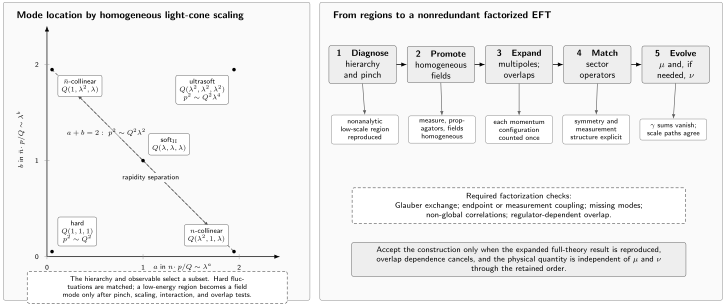
Mode locations are shown in the exponents $a$ and $b$ of $(n\!\cdot p/Q,\bar n\!\cdot p/Q)\sim(\lambda^a,\lambda^b)$, with the transverse exponent written in each label. The line $a+b=2$ contains $n$-collinear, $\bar n$-collinear, and soft-II scalings of virtuality $Q^2\lambda^2$; their separation along the line is a rapidity separation. Ultrasoft momentum has virtuality $Q^2\lambda^4$, while hard fluctuations are matched at $Q^2$. The points are alternatives selected by a hierarchy and observable, not a universal simultaneous field list. A consistent construction requires homogeneous fields, multipole and overlap expansion, sector matching, and $\mu$ and, when needed, $\nu$ evolution, with explicit factorization checks. The diagram is schematic and not to scale.

Failure diagnostics

Uncanceled $1/\eta$ poles. Check that the mode list is complete, the soft and collinear regulator powers are compatible, and every zero-bin has been defined before being evaluated. Changing $\nu$ cannot cancel a missing sector.

A nonzero μ–ν curl. Counterterms, anomalous dimensions, or perturbative orders have been mixed. Compare $D_\mu\gamma_\nu$ with $\partial_{\ln\nu}\gamma_\mu$ sector by sector before solving either evolution equation.

Residual boost or regulator dependence. The physical sector sum is incomplete or has inconsistent Wilson-line orientations and subtractions. Individual functions need not be boost invariant, but the stated observable must be.

Glauber sensitivity. Rapidity-pole cancellation is necessary but not sufficient for factorization. If a pinched Glauber region survives the measurement or cut sum, retain the corresponding operator or restrict the theorem’s scope rather than interpreting it as a regulator artifact.

Exercises

1. Why can ordinary $\mu$ evolution not resum a soft–collinear rapidity logarithm when the modes have equal virtuality?

   Solution

   The modes have the same natural invariant-mass scale and hence the same natural $\mu$, but their ratios $p^+/p^-$ differ parametrically. A second scale conjugate to that boost separation is required.

2. What does a nonzero $(\mu,\nu)$ evolution commutator indicate?

   Solution

   It signals inconsistent anomalous dimensions, regulator counterterms, overlap subtraction, or perturbative truncation. Exact evolution between fixed endpoints cannot depend on the path in the $(\mu,\nu)$ plane.

References

• Altinoluk, Tolga, Guillaume Beuf, and Jani Penttala. 2026. “Exploring Rapidity Regularization Schemes at Low $x$ with the DIS Longitudinal Structure Function.” Journal of High Energy Physics 2026 (4): 125. DOI. Open PDF.

• Chiu, Jui-yu, Ambar Jain, Duff Neill, and Ira Z. Rothstein. 2012. “A Formalism for the Systematic Treatment of Rapidity Logarithms in Quantum Field Theory.” Journal of High Energy Physics 2012 (5): 084. DOI. Open PDF.

• Jaiswal, Prerit, and Takemichi Okui. 2015. “Re-emergence of Rapidity Scale Uncertainty in SCET.” Physical Review D 92 (7): 074035. DOI. Open PDF.

• Li, Ye, Duff Neill, and Hua Xing Zhu. 2020. “An Exponential Regulator for Rapidity Divergences.” Nuclear Physics B 960: 115193. DOI. Open PDF.