Eikonal Approximation and Wilson Lines

A soft gauge field cannot resolve the short-distance structure or recoil of a hard particle at leading power. It sees an oriented classical trajectory carrying charge or color. Algebraically, the hard propagator becomes an eikonal denominator $1/(\beta\cdot k\mp i0)$; repeated emissions exponentiate into a path-ordered Wilson line along the direction $\beta$.

Required background. Soft Theorems supplies the single-emission current. Wilson Lines and Loops defines Wilson operators and their gauge transformation laws.

Helpful background. Parallel Transport and Holonomy gives the geometric interpretation of path ordering and endpoint transport.

The eikonal expansion

Let an on-shell hard momentum be $p=E\beta$, where $\beta$ fixes its direction and need not be normalized. If a soft momentum $k$ enters the adjacent hard line, then

$$(p+k)^2-m^2+i0=2E\,\beta\cdot k+k^2+i0.$$

At $|k|/E\ll1$ this becomes $2E\beta\cdot k+i0$. For a scalar emission,

$$\begin{aligned} &g\mathbf t^a(2p+k)^\mu \frac{1}{(p+k)^2-m^2+i0}\\ &\qquad=g\mathbf t^a\frac{\beta^\mu}{\beta\cdot k+i0} +O(E^{-1}), \end{aligned}$$

where the omitted term is suppressed by $O(k/E)$ relative to the displayed eikonal factor, and up to whether $k$ is defined as entering or leaving the line. For a fermion, the on-shell Dirac equation removes the leading spin dependence and gives the same vector. Spin, recoil, and the $k^2$ term first appear at next-to-eikonal order.

Because momentum-flow choices can obscure the causal sign, we now fix one convention and keep it throughout. Take

$$\begin{aligned} A^a_\mu(x) &=\int\frac{\mathrm d^d k}{(2\pi)^d} e^{-ik\cdot x}A^a_\mu(k),\\ D_\mu&=\partial_\mu-igA_\mu^a\mathbf t^a, \end{aligned}$$

and let $k$ flow from the Wilson line into the gauge field. The outgoing ray from the hard point $0$ is

$$\begin{aligned} W_\beta^{\mathrm{out}}(0) =\mathbf P\exp\!\Bigg[&ig\int_0^\infty \mathrm ds\, \beta\cdot A^a(s\beta)\\ &\times\mathbf t^a\Bigg]. \end{aligned}$$

Its term linear in $A$ gives

$$g\mathbf t^a\frac{\beta^\mu}{\beta\cdot k-i0}.$$

The incoming ray from $-\infty$ to $0$ gives instead

$$-g\mathbf t^a\frac{\beta^\mu}{\beta\cdot k+i0}.$$

Reversing the definition of momentum flow reverses both displayed prescriptions. Physical results are convention independent only if ray orientation, generator representation, and $i0$ signs are changed together. Here $\mathbf t^a$ is the physical-representation generator. If instead all legs are crossed to a common outgoing convention, absorb the ray orientation and conjugate representation into crossed charges $\mathbf T_i^a$ as on the Soft Theorems page; do not retain the explicit incoming minus sign as well.

The reduction is summarized below. The left side retains soft attachments to hard external propagators; the right side keeps only the oriented rays that a soft function needs.

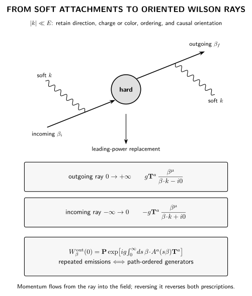
The eikonal limit preserves direction, charge or color, path ordering, and incoming/outgoing causal orientation while discarding leading recoil and spin. The equality is a leading-power replacement for soft interactions, not an equality of complete hard amplitudes; the drawing is schematic.

Path ordering generates multiple emissions

Expanding the exponential to second order produces an ordered integral,

$$\begin{aligned} &(ig)^2\int_0^\infty \mathrm ds_1 \int_0^{s_1}\mathrm ds_2\, \beta\cdot A^{a_1}(s_1\beta)\\ &\qquad\times\beta\cdot A^{a_2}(s_2\beta) \mathbf t^{a_1}\mathbf t^{a_2}. \end{aligned}$$

Fourier transformation yields the individual eikonal poles and a cumulative denominator associated with the ordered sum of soft momenta. In an Abelian theory the charges commute, so ordering is invisible; in a non-Abelian theory it retains the color sequence. This is why a Wilson line, rather than a commuting classical number, is the correct soft source. Schwartz derives the eikonal Feynman rules and ordered exponentiation in Schwartz 2014, § 25.2, printed pp. 488–493.

Under a gauge transformation, an open Wilson line transforms at its two endpoints. A semi-infinite ray is therefore not generally a gauge-invariant operator by itself. In a factorized amplitude, rays meet a hard color tensor, other rays, or specified boundary data so that the complete color contraction has the required gauge covariance or invariance.

Cusps remember relative directions

When two Wilson segments meet with different velocities, their cusp requires renormalization. For timelike directions one may characterize the geometry by

$$\cosh\chi= \frac{\beta_1\cdot\beta_2} {\sqrt{\beta_1^2\beta_2^2}}.$$

The associated cusp anomalous dimension controls the double logarithms of many amplitudes and event shapes. In a lightlike limit, $\chi$ becomes large; if soft and collinear sectors then have equal virtuality, an additional rapidity regulator and scale can be required. Collins, Soper, and Sterman derive the eikonal approximation and explain its role in factorization in Collins, Soper, and Sterman 2004, §§ 8.1–8.4, printed pp. 77–86, PDF.

Domain and failure modes

The eikonal approximation assumes a hierarchy between the soft momentum and the hard particle energy and expands at fixed hard direction. It does not include recoil-sensitive power corrections, spin-dependent subleading soft terms, hard-collinear radiation, or the finite length and structure of a source. Lightlike rays also introduce collinear and sometimes rapidity singularities that must be separated without double counting.

Most importantly, eikonalization does not by itself prove factorization. Momentum in the Glauber region can pinch oppositely directed lines and retain process-dependent color correlations. Whether those exchanges cancel, exponentiate into an allowed operator, or break a proposed factorization formula depends on the process and measurement.

Check your understanding

Expand $W_\beta^{\mathrm{out}}$ to first order and evaluate $\int_0^\infty \mathrm ds\,e^{-is\beta\cdot k}$ with a damping factor $e^{-\delta s}$, $\delta>0$. Verify the denominator $1/(\beta\cdot k-i0)$. Repeat on $s\in(-\infty,0]$ and check that both the overall sign and the $i0$ prescription reverse.

References

• Collins, John C., Davison E. Soper, and George Sterman. “Factorization of Hard Processes in QCD.” In Perturbative Quantum Chromodynamics, edited by A. H. Mueller, 1–91. World Scientific, 1989; updated author manuscript, 2004, esp. §§ 8.1–8.4, printed pp. 77–86. doi:10.1142/9789814503266_0001. Open PDF.
• Schwartz, Matthew D. Quantum Field Theory and the Standard Model. Cambridge University Press, 2014, § 25.2, printed pp. 488–493. doi:10.1017/9781139540940.