Resonance Poles, Riemann Sheets, and Unstable States

An unstable state is defined at amplitude level by a pole on an unphysical Riemann sheet, not by an asymptotic one-particle vector and not by a bump alone. Writing the pole in the complex energy plane as $\sqrt{s_p}=M_p-i\Gamma_p/2$ defines its pole mass and width. Residues factorize among channels, but thresholds, backgrounds, nearby poles, and energy-dependent couplings can move or erase a peak and invalidate a naive Breit–Wigner or narrow-width interpretation.

Required background. Partial-Wave Unitarity supplies $S_\ell$, phase shifts, and inelasticity. Analyticity and Crossing of Amplitudes supplies physical and unphysical sheets. Resonances, Infraparticles, and Limits of Particle Language supplies the warning that an unstable state is not an LSZ external particle.

Helpful background. Poles, Cuts, Thresholds, and Stable Particles and Branches, Sheets, Analytic Continuation, and Monodromy supply spectral and branch-language repair. Cross Sections and Decay Rates supplies the observable normalization.

One channel in the momentum plane

For two equal-mass particles, define

$$k(s)=\frac12\sqrt{s-4m^2}.$$

The square root produces two $s$-plane sheets. The physical sheet maps to $\operatorname{Im}k>0$, and crossing the elastic cut maps to $\operatorname{Im}k<0$. In this convention:

• a bound-state pole has $k=i\kappa$, $\kappa>0$, on the physical sheet below threshold;
• a virtual-state pole has $k=-i\kappa$ on the unphysical sheet below threshold; and
• a resonance pole lies off the imaginary axis on a channel-adjacent unphysical sheet, with the decaying pole in the lower half of the complex energy plane.

For multiple two-body channels, every channel momentum contributes a square-root sign choice. “The second sheet” is therefore insufficient: the sheet must be labeled by all sign choices and by which physical energy interval it borders. Particle Data Group 2025, review 50, § 50.1.1, printed pp. 3–7, PDF gives the one- and two-channel mappings and emphasizes that sheet proximity changes across thresholds.

An effective-range model shows why a near-threshold line shape does not by itself distinguish the first two cases. Adopt the convention

$$f_0(k)=\frac{1}{k\cot\delta_0-ik}, \qquad k\cot\delta_0=-\frac1a+\frac12r_e k^2+O(k^4).$$

Neglecting $r_e$ gives a pole at $k=i/a$. Thus $a>0$ places a shallow bound state at $+i/a$, while $a<0$ places a virtual state at $-i/|a|$ on the adjacent sheet. Nevertheless,

$$|f_0(k)|^2=\frac{1}{a^{-2}+k^2}$$

is identical for $a$ and $-a$ on the physical axis. The sheet location, not the intensity alone, distinguishes the states. Some communities define the leading term with the opposite sign; translate the pole position before translating the label “positive scattering length.”

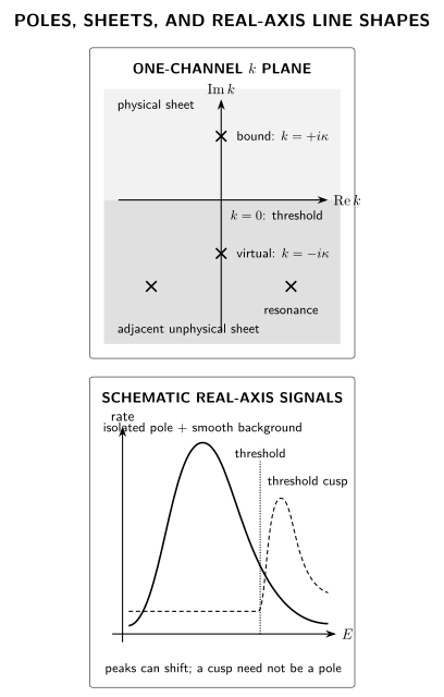
The $k$-plane removes the single elastic square-root cut and separates bound, virtual, and resonance poles by half-plane. The line shapes are schematic and not to scale: background interference or a threshold cusp can shift, hide, or mimic a peak without changing the pole classification.

Pole position and residue

Near an isolated resonance pole,

$$\begin{aligned} \mathcal T_{ij}(s) &=\frac{r_{ij}}{s-s_p}+\mathcal T_{ij}^{\mathrm{reg}}(s),\\ r_{ij}&=g_i^{\mathrm{out}}g_j^{\mathrm{in}}. \end{aligned}$$

where the phases and normalization of the channel couplings depend on conventions. In a time-reversal-invariant basis the residue matrix is symmetric and can be written $r_{ij}=g_i g_j$. The pole position is shared by every amplitude that couples to that pole; unlike a peak position, it does not depend on the chosen production process. Write

$$\sqrt{s_p}=M_p-\frac{i}{2}\Gamma_p, \qquad \Gamma_p>0.$$

Here the square root is the branch with positive real part continued to the pole. The pole definition of mass and width, together with the distinction between exact pole data and Breit–Wigner approximations, is derived in Willenbrock 2024, §§ 2–3, eqs. (11) and (15)–(19).

This definition remains meaningful when a real-axis peak is asymmetric or absent. The residue factorizes for an isolated simple pole, although its channel couplings can be complex and are not probabilities by themselves. The 2025 PDG review distinguishes pole parameters from Breit–Wigner and line-shape quantities and records the correction status for the current edition on the official errata page.

An old but useful narrow-resonance derivation follows from unitarity: near a single isolated level with slowly varying background, the denominator takes the form $E-E_R+i\Gamma/2$. Weinberg derives that limit and its phase-shift motion in Weinberg 1995, § 3.8, printed pp. 159–165. The derivation does not make the approximation reliable near every modern coupled-channel threshold.

When a Breit–Wigner description works

A simple line shape may be written schematically as

$$\mathcal T(s) \simeq \frac{N(s)}{M_{\mathrm{BW}}^2-s-iM_{\mathrm{BW}}\Gamma(s)}+B(s).$$

Identifying $M_{\mathrm{BW}}$, a peak location, and $M_p$ requires all of the following to be controlled:

• the pole is isolated and narrow compared with its mass and the nearest variation scale;
• $N(s)$, $\Gamma(s)$, phase space, and background $B(s)$ vary slowly across the resonance region;
• no nearby threshold, zero, cusp, or second pole dominates;
• interference with nonresonant and neighboring resonant amplitudes is small or modeled coherently; and
• the chosen parametrization respects the coupled-channel analytic and unitarity structure.

If these conditions fail, a bump can be displaced, a resonance can appear as a dip, a threshold can make a cusp without a nearby resonance pole, and a pole can exist without a conspicuous bump. The PDG review gives explicit sheet and threshold examples in Particle Data Group 2025, review 50, § 50.1.1, printed pp. 3–7, PDF.

Narrow-width factorization and gauge limitations

For an inclusive observable dominated by one isolated pole, the squared propagator has the distributional limit

$$\begin{aligned} &\frac{1}{(s-M^2)^2+M^2\Gamma^2}\\ &\quad\xrightarrow[\Gamma/M\to0]{} \frac{\pi}{M\Gamma}\,\delta(s-M^2). \end{aligned}$$

This can factorize production and decay after the phase space and matrix elements are shown to be smooth over the width. It fails for sharp cuts, strong interference, nonfactorizable corrections, overlapping resonances, and near-threshold poles. In gauge theories, inserting a width into only a selected propagator resums some loop terms but not the Ward-related set; a controlled pole expansion or gauge-consistent unstable-particle scheme is needed. The later page on unstable-particle observables and resonance approximations develops the controlled observable-level continuation. Process-specific hadron and electroweak resonances belong to their specialist volumes, and current fits belong in Research.

Check your understanding

Place poles at $k=+i\kappa$, $-i\kappa$, and $k_R-i\gamma$, map each to its $s$-sheet, and state which can represent an asymptotic stable particle. Then list two mechanisms that move a real-axis peak away from $\operatorname{Re}\sqrt{s_p}$. The check passes only if a threshold cusp is not automatically called a resonance.

Solution

$+i\kappa$ is a physical-sheet pole below threshold and can be a stable bound state. $-i\kappa$ is a virtual-state pole on the adjacent sheet and is not an asymptotic one-particle state. $k_R-i\gamma$ is an off-axis adjacent-sheet resonance pole. A rapidly varying threshold factor and interference with a regular background can both shift or erase the peak; a nearby zero or another pole provides further mechanisms. A cusp at $k=0$ can arise from the branch point without any nearby pole.

References

• Particle Data Group. “Resonances.” In Review of Particle Physics, 2025 Update, review 50, especially §§ 50.1.1–50.1.3, printed pp. 3–13. Official PDF. Official errata.
• Weinberg, Steven. The Quantum Theory of Fields, Volume I: Foundations. Cambridge University Press, 1995, § 3.8, printed pp. 159–165. doi:10.1017/CBO9781139644167.
• Willenbrock, Scott. “Mass and Width of an Unstable Particle.” European Physical Journal Plus 139 (2024): article 523. doi:10.1140/epjp/s13360-024-05301-0; Open PDF.