

Singularities, Vanishing Cycles, and Monodromies
A Coulomb-branch singularity occurs when the photon-only effective theory omits a state whose central charge vanishes. For one primitive mutually local BPS hypermultiplet, its logarithmic threshold determines an integral Picard–Lefschetz monodromy. The set of local monodromies, based paths, and their ordered product constrains the global special geometry.
Required background. Charge local systems and duality frames fixes transport conventions, and singular loci and light fields fixes the EFT interpretation. Helpful background. Branches and monodromy supplies the analytic-continuation language.
Local behavior near a massless hypermultiplet
Section titled “Local behavior near a massless hypermultiplet”Choose a duality frame in which the light charge is electric and let its special coordinate be . Integrating out one charged hypermultiplet produces a logarithmic coupling. In a rank-one normalization appropriate to pure , a monopole point can be written locally as
and
A counterclockwise loop sends , so
Thus, for the period column ,
The factor two belongs to the non-unimodular particle polarization used for the pure- benchmark. In the chapter’s root-unit labels the massive boson is , while
Equivalently one may use weight-unit electric labels with , but then , every charge, and every matrix must be conjugated together. A simple unimodular Lefschetz degeneration can have coefficient one; it is not the convention used by the matrices below.
Monodromy from a vanishing charge
Section titled “Monodromy from a vanishing charge”Let
In the root-unit rank-one convention above, the monodromy acting on periods is
It is integral, has determinant one, and preserves . Moreover,
so the vanishing period is single-valued around its own singularity.
Changing the charge basis conjugates . Reversing the loop inverts it. Replacing by leaves the matrix unchanged, as expected because a particle and antiparticle become massless together.
For several mutually local hypermultiplets of the same primitive charge, the coefficient is multiplied by their net protected contribution. A massless vector multiplet produces a different threshold sign and signals restored nonabelian gauge symmetry; do not use the hypermultiplet formula blindly.
Vanishing cycles
Section titled “Vanishing cycles”In a curve description, charges correspond to one-cycles, but the curve intersection and physical particle pairing need a polarization crosswalk. For a simple Lefschetz degeneration in a unimodular homology basis, transport around the primitive shrinking cycle acts on another cycle by
in a unit-intersection convention, with orientation-dependent sign. Integrating the Seiberg–Witten differential over the transported cycles gives the period monodromy.
At each finite singularity, the pure- family below has an Kodaira degeneration whose monodromy lies in , as appropriate to its adjoint particle polarization. With and ,
Thus the geometric formula and the one-loop threshold agree only after the sign and factor-two translation. This is an independent check, not a convention to infer after seeing the desired matrix.
Pure SU(2): two finite singularities
Section titled “Pure SU(2): two finite singularities”Use the chapter’s frozen pure- convention: , weak-coupling base point , period column , and
whose discriminant has finite zeros at . Let and be the counterclockwise based meridians shown in the figure below, with the stem for the negative point transported through the declared upper-half-plane path. Define loop-word multiplication and the monodromy representation so that
Period matrices act on columns from the left; consequently the rightmost matrix in a written product is applied first. This declaration removes the usual ambiguity between path traversal, loop words, and operator composition.
Assign a monopole charge
at and a dyon charge
at . The matrices are
With the convention that the based loop at infinity corresponds to the ordered product ,
This agrees with the semiclassical logarithm. The physical pairing of the two transported light charges is . A different cut system can exchange the dyon label or conjugate all three matrices; the based product must still match the transformed infinity monodromy. The singularity assignment and global monodromy product are derived in Seiberg and Witten 1994, §§5–6 and reconstructed with explicit continuation conventions in Bilal 1996, §§5–6.
The shared figure freezes the cycle basis, based loops, particle-pairing translation, strong- and weak-chamber data, and the later small- deformation in one record. Inspect the loop labels before comparing matrix products, and inspect the stop rule before carrying the confinement picture away from the controlled regime.
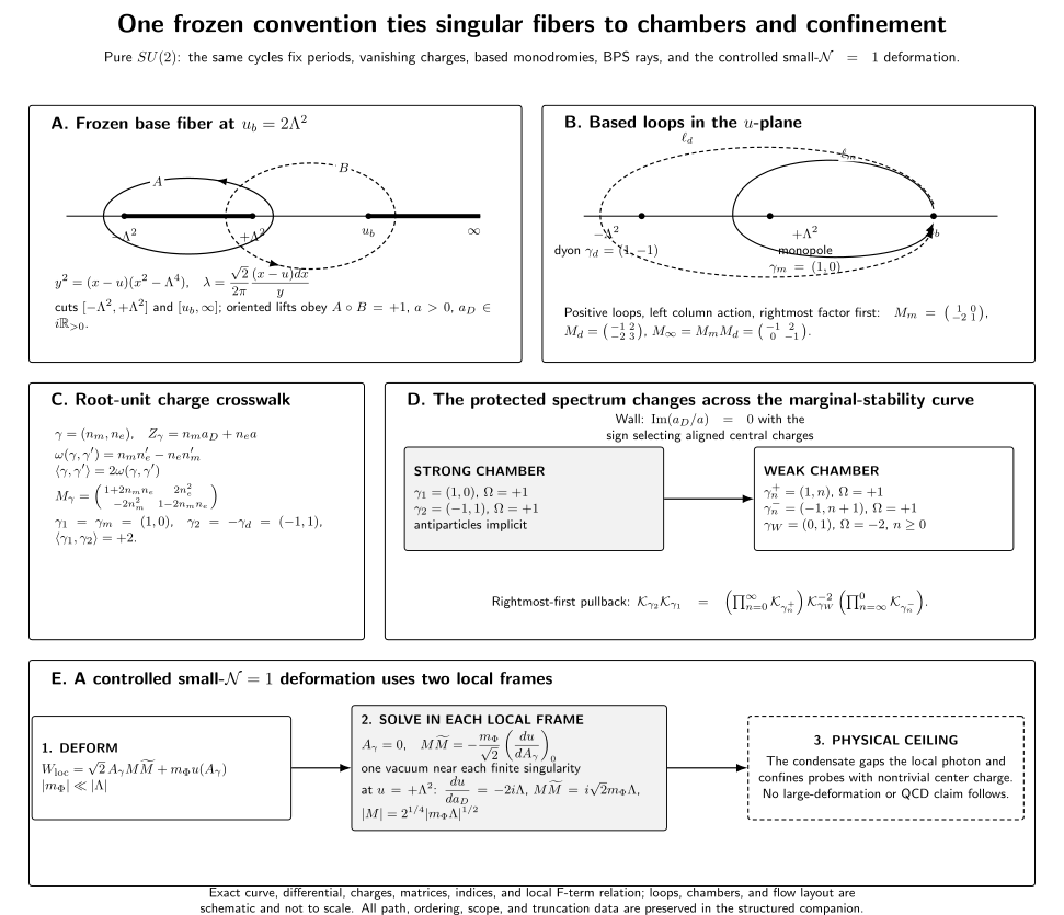
For and , the root-unit particle labels have and physical pairing . The and transported combinations give and ; the declared based-loop convention gives , with the rightmost matrix applied first. The chamber and panels are conditional on their displayed half-plane and hierarchy. Exact matrices, period fixtures, the corrected wall-crossing order, F-terms, and limitations are in the structured rank-one record.
Discriminant completeness
Section titled “Discriminant completeness”For a proposed curve, compute its discriminant as a function of Coulomb moduli and masses. Every zero is a candidate singular fiber, but multiplicity alone does not identify the light theory. One must determine:
- which cycle or set of cycles vanishes;
- whether each charge is primitive;
- their pairwise Dirac pairings;
- the local order of vanishing of periods;
- whether the singularity lies at finite distance;
- whether a weakly coupled electric frame exists.
Missing a discriminant component makes the global monodromy product fail. Adding a spurious component produces an unphysical light sector or incorrect asymptotics.
Mutually nonlocal collisions
Section titled “Mutually nonlocal collisions”Suppose two discriminant components collide and their vanishing charges satisfy
No electric frame contains both as local hypermultiplets. The collision can yield an interacting Argyres–Douglas fixed point. The product of local monodromies remains integral, but a sum of two weakly coupled QED logarithms is not a valid local description at the collision.
Scaling dimensions must then be extracted from the degenerating curve and differential, with . Existence of an interacting fixed point also requires consistent unitarity and protected data.
Global consistency procedure
Section titled “Global consistency procedure”- Choose a base point and a symplectic charge basis.
- Specify branch cuts and oriented loop generators.
- Compute the complete discriminant.
- Determine each vanishing charge in the base-point frame.
- Construct local monodromies and verify integrality and symplecticity.
- Multiply them in the declared path order.
- Compare with the independently derived monodromy at infinity.
- Transform charges by the inverse transpose and verify central-charge invariance.
The global product is a stringent check because local sign errors can preserve each determinant while failing the total monodromy.
Common pitfalls
Section titled “Common pitfalls”Naming a vanishing charge without a path. Transport from the singularity to the base point is part of its charge label.
Multiplying matrices in an undeclared order. Loop composition and active action conventions determine whether or is correct.
Using the hypermultiplet formula at a mutually nonlocal collision. There is no single local electric QED frame there.
Exercises
Section titled “Exercises”Starting only from the charge formula and the declared paths:
- reconstruct and ;
- compute the geometric determinant and physical pairing of and ;
- verify and ;
- explain how an arbitrary transported charge must transform when .
Solution
Substitution of and gives the displayed matrices. Their coordinate determinant is
so their physical particle pairing is . Both determinants equal one, and matrix multiplication gives
Finally,
Thus each vanishing central charge is invariant around its own singularity.
For a general charge column , the same physical state is represented after continuation by . Therefore
References
Section titled “References”- Bilal, Adel. “Duality in SUSY Yang–Mills Theory: A Pedagogical Introduction to the Work of Seiberg and Witten.” 1996. arXiv:hep-th/9601007.
- Seiberg, Nathan, and Edward Witten. “Electric–Magnetic Duality, Monopole Condensation, and Confinement in Supersymmetric Yang–Mills Theory.” Nuclear Physics B 426 (1994): 19–52; erratum 430 (1994): 485–486. arXiv:hep-th/9407087.
Further reading
Section titled “Further reading”- Picard, Émile, and Georges Simart. Théorie des fonctions algébriques de deux variables indépendantes, vol. 2. Gauthier-Villars, 1906.