Forward-Limit Positivity Bounds

For a gapped elastic channel with a finite forward limit, real analyticity, crossing, unitarity, and sufficiently mild complex-energy growth imply that the even derivatives of the pole-subtracted forward amplitude are positive. The conclusion is a theorem about this package of hypotheses, not about an arbitrary low-energy Lagrangian in isolation.

Required background. Forward scattering sum rules supplies the absorptive moments. Causality, growth, and analytic domains supplies the high-energy and domain assumptions that close the contour.

Forward positivity theorem

Let $A(s,t)$ describe identical scalar particles of mass $m$. Define $v=s-2m^2$ at $t=0$ and remove every known stable $s$- and $u$-channel pole to obtain $B(v)$. Assume:

1. $B(v)$ is real analytic in the complex $v$-plane cut only for $|v|\ge\nu_0$, with $\nu_0=2m^2$ for the two-particle threshold.
2. Crossing gives $B(v)=B(-v)$.
3. The large-arc estimate $B(v)/v^2\to0$ holds in the cut plane.
4. The forward optical theorem gives $\rho(\nu)=\operatorname{Im}A(2m^2+\nu+i0,0)\ge0$.
5. The dispersive integrals converge and no massless pole or cut pinches $t=0$.

Then, for every $n\ge1$,

$$\boxed{ \frac{B^{(2n)}(0)}{(2n)!} =\frac{2}{\pi}\int_{\nu_0}^{\infty} \frac{\rho(\nu)}{\nu^{2n+1}}\,\mathrm d\nu\ge0 }$$

The inequality is strict provided the chosen initial state has nonzero absorptive weight at finite energy. If it is completely decoupled, the theorem gives only nonnegativity. The contour proof and the original EFT sign application appear in Adams et al. 2006, § 4, pp. 14–19, PDF; the gapped scalar assumptions and pole-subtracted formulation are sharpened in de Rham et al. 2017, pp. 1–4, PDF.

Each assumption has a separate job. Analyticity produces the integral, the growth bound fixes two subtractions, crossing gives the same sign for both cuts, and unitarity supplies $\rho\ge0$. Removing any one of those inputs need not make the amplitude inconsistent; it makes this conclusion unavailable.

More than one positive coefficient

Set

$$c_{2n}=\frac{B^{(2n)}(0)}{(2n)!}.$$

The coefficients form a moment sequence. Cauchy–Schwarz and the lower endpoint of the cut imply

$$c_{2n+2}^2\le c_{2n}c_{2n+4}, \qquad 0\le c_{2n+2}\le\frac{c_{2n}}{\nu_0^2}.$$

The lower inequality is strict under the same nonzero-spectral-weight condition stated above.

To see the geometry, use the positive measure proportional to $\rho(\nu)\nu^{-3}\mathrm d\nu$ and set $x=\nu^{-2}\in[0,X]$, $X=\nu_0^{-2}$. With moments $m_k=\int x^k\mathrm d\mu$, define

$$r=\frac{m_1}{Xm_0}, \qquad q=\frac{m_2}{X^2m_0}.$$

Positivity and compact support give $0\le r\le1$ and

$$r^2\le q\le r.$$

The lower curve is saturated by spectral weight at one scale; positive mixtures fill the region. Inspect the two boundaries in the figure rather than only the shaded interior.

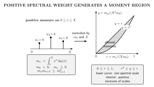
Schematic positive-moment construction. With $x=\nu^{-2}\in[0,X]$ and $\mathrm d\mu\ge0$, normalized moments obey $r^2\le q\le r$. A single spectral scale lies on the lower parabola, while positive mixtures lie on or inside the shaded region; no color distinction is required and the axes are dimensionless.

Figure quantity	Amplitude meaning
$m_0,m_1,m_2$	three successive positive forward derivative moments
$r^2\le q$	$2\times2$ Hankel positivity, or Cauchy–Schwarz
$q\le r$	the spectral support satisfies $0\le x\le X$
lower parabola	one spectral value of $x$; a narrow-resonance idealization
shaded interior	positive superpositions of more than one scale

The general positive-moment and finite-Hankel formulation is developed in Bellazzini et al. 2021, § I.A–B, pp. 2–5, PDF.

A scalar EFT coefficient

Suppose the pole-subtracted low-energy amplitude has the crossing-symmetric expansion

$$B(s,t)=\frac{g_2}{\Lambda^4}(s^2+t^2+u^2) +O\!\left(\frac{p^6}{\Lambda^6}\right) +B_{\mathrm{light\ loops}}(s,t).$$

At $t=0$, use $s=2m^2+v$ and $u=2m^2-v$. The mass-dependent part of $s^2+u^2$ is independent of $v$, so

$$B(v,0)=\text{constant}+\frac{2g_2}{\Lambda^4}v^2+\cdots.$$

At tree level, with light-loop pieces negligible at the stated order, the theorem gives $g_2>0$. This is an amplitude-level statement. The numerical relation between $g_2$ and a Lagrangian Wilson coefficient depends on operator normalization, integrations by parts, equations of motion, and field redefinitions.

Once light loops matter, $B^{(2)}(0)$ contains both local coefficients and the Taylor contribution of low-energy loops, whose global nonanalyticity is encoded in light cuts. One must either retain the complete physical combination or subtract a calculable low-energy absorptive integral consistently. The sign of a running coefficient by itself is not generally the theorem.

A heavy-threshold field-theory check

Let a light real scalar $\phi$ couple to a heavier real scalar $\chi$ through

$$\mathcal L_{\mathrm{int}}=-\frac{\lambda}{4}\phi^2\chi^2, \qquad M_\chi=M>m_\phi=m.$$

At order $\lambda^2$, the crossing-symmetric heavy bubble gives a forward coefficient

$$c_2^{(\chi)} =\frac{\lambda^2}{32\pi^2} \int_0^1\mathrm dx\, \frac{x^2(1-x)^2} {[M^2-2m^2x(1-x)]^2}>0.$$

For $M\gg m$,

$$c_2^{(\chi)} =\frac{\lambda^2}{960\pi^2M^4} \left[1+\frac67\frac{m^2}{M^2}+O\!\left(\frac{m^4}{M^4}\right)\right].$$

The same sign follows independently from the cut, $\operatorname{Im}\mathcal M(s,0)=\lambda^2\sqrt{1-4M^2/s}/(32\pi)$ for $s\ge4M^2$, inserted into the positive forward moment. The example checks the loop symmetry factor, threshold support, optical-theorem normalization, and low-energy coefficient; it is a perturbative heavy-threshold test, not a proof of an all-scale UV completion.

Failure modes

Insufficient subtractions. If $B/v^2$ does not vanish, the large arc can contribute and the displayed equality is incomplete. Adding a subtraction may protect the contour but also turns the targeted derivative into subtraction data.

Wrong crossing sector. For multiple species or spin, crossing is a matrix. A component amplitude need not inherit the positive eigenvalue used above.

Unsubtracted poles. A stable exchange term can dominate the Taylor coefficient without contributing to the continuum integral. Remove it with the same sign and normalization as in the amplitude.

No forward analytic neighborhood. Massless exchange produces $1/t$ poles and loops can produce $\log(-t)$. The theorem then cannot be applied by simply setting $t=0$.

Overstated conclusion. Passing these inequalities is necessary for the declared completion class, not sufficient to construct or prove a UV completion.

Exercises

Suppose $c_2=1$ and the threshold unit is chosen so that $\nu_0=1$. Which pairs $(c_4,c_6)$ are ruled out by the first support and Hankel tests?

Check

They must satisfy $0<c_4\le1$, $0<c_6\le c_4$, and $c_6\ge c_4^2$. For example, $(c_4,c_6)=(1/2,1/10)$ fails Hankel positivity, while $(1/2,3/4)$ fails the support bound.

Strengthen the constraints: Beyond-Forward Positivity. If the forward limit is singular: Massless Exchange and Infrared Subtractions.

References

• Adams, Allan, Nima Arkani-Hamed, Sergei Dubovsky, Alberto Nicolis, and Riccardo Rattazzi. “Causality, Analyticity and an IR Obstruction to UV Completion.” Journal of High Energy Physics 10 (2006): 014. DOI. Open PDF.
• Bellazzini, Brando, Joan Elias Miró, Riccardo Rattazzi, Marc Riembau, and Francesco Riva. “Positive Moments for Scattering Amplitudes.” Physical Review D 104 (2021): 036006. DOI. Open PDF.
• de Rham, Claudia, Scott Melville, Andrew J. Tolley, and Shuang-Yong Zhou. “Positivity Bounds for Scalar Theories.” Physical Review D 96 (2017): 081702. DOI. Open PDF.