Unstable-Particle Observables and Controlled Resonance Approximations

An unstable excitation is observed through stable decay products, not as an exact asymptotic particle. Near a resonance, amplitudes may nevertheless be expanded around a gauge-invariant complex pole. Pole, double-pole, and narrow-width approximations are controlled only when their small parameter, retained spin correlations, nonresonant terms, cuts, and perturbative order are stated together.

Required background. Cross Sections and Decay Rates supplies stable-final-state phase space. Resonance Poles, Riemann Sheets, and Unstable States supplies the complex pole and sheet structure. Fixed-Order Organization and Scale Dependence supplies the perturbative counting used for widths and corrections.

Helpful background. LSZ Reduction: Poles, Residues, and Stable External States explains why a finite-width state is not an LSZ external leg. Partial-Wave Unitarity provides the elastic resonance context. Resummation and Fixed-Order Matching supplies the general logic of combining expansions without double counting.

Stable final states and the complex pole

Consider a process $a b\to f$, where every particle in $f$ is stable on the scattering time scale. If a subset has invariant mass $s$, the amplitude near an isolated resonance can be written

$$\mathcal M_{ab\to f}(s) =\frac{R_{ab\to f}(s_\star)}{s-s_\star} +N_{ab\to f}(s),$$

where

$$s_\star=M_\star^2-iM_\star\Gamma_\star$$

is the pole on the appropriate unphysical sheet. The pole position and properly defined residue are gauge independent, whereas an arbitrary separation into selected resonant diagrams and a background generally is not. Pole-based organization of gauge-invariant resonance parameters is established in Stuart 1991, pp. 113–119.

$M_\star$ and $\Gamma_\star$ are pole parameters. A Breit–Wigner fit with a running width, a real-axis on-shell mass, or a threshold-distorted line shape can use different parameters. These conventions should not be equated without an explicit translation.

The figure below distinguishes the analytic pole data from real-axis line shapes. Inspect in particular that a resonance pole lies on a connected unphysical sheet and that a nearby threshold can make the observed peak asymmetric or move it away from $\operatorname{Re}s_\star$.

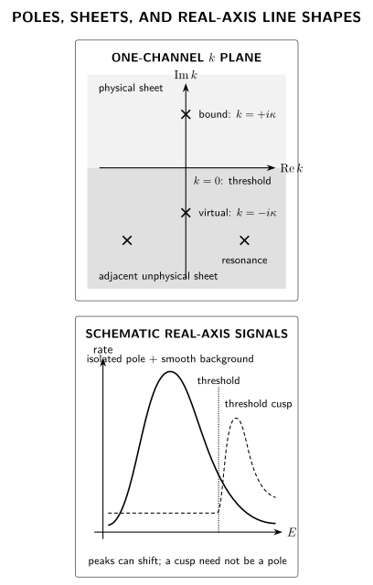
Pole locations and observable line shapes. Bound, virtual, and resonant states are distinguished by sheet and pole position; a Breit–Wigner-like peak is only a real-axis approximation and may be distorted near thresholds. The diagram is schematic and not to scale.

Narrow-width approximation

For $\Gamma_\star/M_\star\ll1$ and a smooth test function $f(s)$,

$$\begin{aligned} &\int \mathrm ds\, \frac{f(s)}{(s-M_\star^2)^2+M_\star^2\Gamma_\star^2}\\ &\qquad\longrightarrow \frac{\pi}{M_\star\Gamma_\star}f(M_\star^2). \end{aligned}$$

Equivalently,

$$\begin{aligned} \frac{1}{(s-M^2)^2+M^2\Gamma^2} &\xrightarrow[\Gamma/M\to0]{}\\ &\frac{\pi}{M\Gamma}\,\delta(s-M^2) \end{aligned}$$

as a distribution. This yields the familiar inclusive factorization

$$\begin{aligned} \sigma(a b\to R\to f) &\simeq \sigma(a b\to R)\\ &\quad\times\operatorname{Br}(R\to f). \end{aligned}$$

Here $\sigma(a b\to R)$ is the on-shell projected production factor defined within the narrow-width approximation, not an exact observable with $R$ as an external state.

The last equation suppresses spin indices. For differential observables, production and decay are connected by a spin-density matrix,

$$\mathrm d\sigma \propto \sum_{\lambda,\lambda'} \rho^{\mathrm{prod}}_{\lambda\lambda'} \rho^{\mathrm{dec}}_{\lambda'\lambda} \mathrm d\Phi_{\mathrm{prod}}\,\mathrm d\Phi_{\mathrm{dec}}.$$

Replacing this contraction by independent spin averages destroys angular correlations. The accuracy of decorrelated and spin-correlated narrow-width approximations depends on inclusiveness and kinematic boundaries; a systematic analysis is given in Uhlemann and Kauer 2009, open-manuscript PDF, §§ II–III, pp. 3–16.

When the approximation is controlled

The usual relative estimate $O(\Gamma/M)$ assumes more than a small width. It can fail or be enhanced when:

• the measurement function or parton luminosity varies appreciably across the resonant region;
• a phase-space threshold or endpoint lies within $O(M\Gamma)$;
• another pole overlaps the resonance;
• nonresonant amplitudes are not parametrically suppressed;
• destructive interference makes the nominal leading resonant term small;
• cuts select an off-shell tail;
• the observable is sensitive to soft exchange connecting production and decay.

The correct expansion parameter is tied to the observable and its kinematic region, not only to a particle-property table.

For two resonant propagators, a double-pole approximation retains the leading term near both complex poles. It is appropriate only where both reconstructed invariants lie in their resonant regions. Outside that domain, singly resonant and nonresonant terms can be of the same order.

Gauge and perturbative consistency

In a weakly coupled theory, $\Gamma/M$ is itself of order a coupling squared. Resumming a self-energy into

$$\frac{1}{s-M_0^2+\Sigma(s)}$$

while truncating vertices and nonresonant diagrams inconsistently can mix perturbative orders and violate Ward identities. A controlled calculation specifies whether it uses a pole expansion, complex-mass scheme, or another gauge-consistent organization, and expands production, decay, width, and branching ratios coherently.

If

$$\Gamma=\Gamma_0+\alpha\Gamma_1+\cdots,$$

putting a higher-order width into a nominally lower-order denominator imports selected higher-order terms. That choice may be useful, but its impact must be counted and not combined again as a separate correction. Aeppli, van Oldenborgh, and Wyler organize one-loop resonance calculations around gauge-invariant pole residues in Aeppli, van Oldenborgh, and Wyler 1994, § 4, pp. 131–133; §§ 7–8, pp. 141–143. The pole scheme, pole approximation, complex-mass scheme, and their respective gauge-consistency domains are reviewed in Denner and Dittmaier 2020, §§ 6.1–6.7, pp. 122–147.

Interference and validation

Write the stable-final-state amplitude as $\mathcal M=\mathcal M_{\mathrm{pole}}+\mathcal M_{\mathrm{nonres}}$. The cross section contains

$$\begin{aligned} |\mathcal M|^2={}&|\mathcal M_{\mathrm{pole}}|^2\\ &+2\operatorname{Re}(\mathcal M_{\mathrm{pole}} \mathcal M_{\mathrm{nonres}}^*)\\ &+|\mathcal M_{\mathrm{nonres}}|^2. \end{aligned}$$

Dropping the last two terms is an approximation, not a definition of signal. Validate it by varying the invariant-mass window, comparing the pole-expanded and full stable-final-state calculation at a lower order, checking gauge-parameter independence, and preserving spin correlations. The reusable validation matrix lists these checks alongside scale, pole, numerical, and limiting-case tests.

Common pitfalls

Using an unstable particle as an external LSZ state. The observable is defined on stable decay products. The resonance appears as an internal pole.

Selecting “resonant diagrams” as a gauge-invariant signal. Diagram subsets generally depend on gauge and field parametrization. Use pole residues or another explicitly gauge-consistent scheme.

Applying the delta-function limit through a sharp threshold or cut. The test function must be smooth over the width scale. Check the actual measurement and phase-space boundaries.

Dropping spin correlations in a differential observable. Retain the production–decay density-matrix contraction unless decorrelation has been justified for the measured quantity.

Check your understanding

Integrate the Lorentzian over the entire real line and recover $\pi/(M\Gamma)$. Then choose a test function with a step at $s=M^2$ and explain why replacing it by its value at the pole is ambiguous, exposing the smoothness assumption behind the narrow-width limit.

Where to continue

• Validation and Theory Uncertainties supplies the reusable gauge, pole, scale, and benchmark checks.
• Resonance Poles, Riemann Sheets, and Unstable States develops the analytic continuation underlying $s_\star$.
• Measurement Functions and Inclusive Observables makes invariant-mass windows and stable-final-state cuts explicit.
• Unstable-Particle Effective Theory organizes resonant and nonresonant modes in a systematic width expansion.
• Standard Model Pseudo-Observables and Unstable Particles develops process-level electroweak applications.

References

• Aeppli, André, Geert Jan van Oldenborgh, and Daniel Wyler. “Unstable Particles in One-Loop Calculations.” Nuclear Physics B 428 (1994): 126–146. DOI. Open preprint.
• Denner, Ansgar, and Stefan Dittmaier. “Electroweak Radiative Corrections for Collider Physics.” Physics Reports 864 (2020): 1–163. DOI. Open preprint.
• Stuart, Robin G. “Gauge Invariance, Analyticity and Physical Observables at the $Z^0$ Resonance.” Physics Letters B 262 (1991): 113–119. DOI.
• Uhlemann, Christian F., and Nikolas Kauer. “Narrow-Width Approximation Accuracy.” Nuclear Physics B 814 (2009): 195–211. DOI. Open PDF.