Expansion by Regions

Expansion by regions constructs an asymptotic series by assigning homogeneous scalings to loop momenta, Taylor-expanding the integrand in each scaling, and integrating every expanded term over the full regulated domain. The sum can reproduce powers and logarithms that no single Taylor expansion sees. Its validity depends on the declared limit, a complete set of regions, compatible regulators, and an independent check.

Required background. Anatomy of a Loop Integral supplies the momentum-region and pinch diagnosis; Feynman and Schwinger Parameters supplies an alternative geometric representation; and Dimensional Regularization as an Amplitude Tool supplies the regulator that makes many overlap terms scaleless.

Helpful background. One-Loop Integral Families and Analytic Functions provides exact functions against which expansions can be checked; Tensor Reduction helps organize numerator power counting; and Asymptotic Scales, Remainders, and Uniformity supplies the meaning of an ordered asymptotic series.

A region is a scaling, not a cutoff domain

Let $\lambda\ll1$ describe a hierarchy such as $m/Q\sim\lambda$. A candidate region assigns a homogeneous scaling to every loop-momentum component. Examples include

$$k_{\mathrm h}^\mu\sim Q, \qquad k_{\mathrm s}^\mu\sim \lambda Q,$$

and, for null reference directions normalized by $n^2=\bar n^2=0$ and $n\mathbin{\cdot}\bar n=2$,

$$(n\cdot k_{\mathrm c},\bar n\cdot k_{\mathrm c},k_{\mathrm c\perp}) \sim Q(\lambda^2,1,\lambda).$$

Near a nonrelativistic threshold, potential momenta instead have $k^0\sim mv^2$ and $|\mathbf k|\sim mv$. These are distinct homogeneous expansions; “small momentum” is too vague to identify them.

The operational rule is:

1. state the external scaling, sheet, and regulators;
2. identify scalings in which a consistent set of denominators becomes small;
3. Taylor-expand each integrand according to its scaling;
4. integrate every expanded term over the full loop-momentum domain;
5. sum the regions at fixed order in $\lambda$; and
6. compare with an exact representation, differential equation, or numerical result.

Extending each expansion over the full domain creates apparent overlaps. In pure dimensional regularization many overlap integrals have no scale and vanish; with analytic, rapidity, or cutoff regulators, overlap subtractions may be explicit. The general prescription and the need for care outside proven cases are discussed in Semenova, Smirnov, and Smirnov 2019, §§1–2, pp. 1–4.

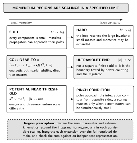
The method expands in homogeneous momentum scalings selected by the external hierarchy. The diagram is schematic and not to scale; not every displayed region contributes to a given limit, and a contour or parameter analysis is needed to establish completeness.

A two-mass example

Consider the Euclidean integral

$$J(M,m)=\mu^{2\epsilon}\int\frac{\mathrm d^d k}{(2\pi)^d} \frac{1}{(k^2+M^2)(k^2+m^2)}, \qquad m\ll M.$$

Its exact partial fraction is

$$J(M,m)=\frac{T_E(m^2)-T_E(M^2)}{M^2-m^2},$$

where

$$T_E(a)=\mu^{2\epsilon}\int\frac{\mathrm d^d k}{(2\pi)^d} \frac{1}{k^2+a} =\frac{\mu^{2\epsilon}}{(4\pi)^{d/2}} \Gamma\!\left(1-\frac d2\right)a^{d/2-1}.$$

Thus, with $r=m^2/M^2$ and $d=4-2\epsilon$,

$$J(M,m)= \frac{\mu^{2\epsilon}}{(4\pi)^{d/2}} \Gamma\!\left(1-\frac d2\right)M^{-2\epsilon} \frac{r^{1-\epsilon}-1}{1-r}.$$

The two distinct small-$r$ series, $-(1+r+\cdots)$ and $r^{1-\epsilon}(1+r+\cdots)$, are the hard and soft contributions. The exact expression therefore supplies an independent expansion target rather than merely a dimensional check.

In the hard region $k\sim M$, expand the light propagator:

$$\frac{1}{k^2+m^2} =\frac1{k^2}\left(1-\frac{m^2}{k^2}+\cdots\right),$$

while retaining $k^2+M^2$. In the soft region $k\sim m$, expand

$$\frac{1}{k^2+M^2} =\frac1{M^2}\left(1-\frac{k^2}{M^2}+\cdots\right),$$

while retaining $k^2+m^2$. Starting beyond leading order, hard terms can develop IR poles while soft terms carry UV poles; their regulated sum has the pole structure of the original two-scale integral. The common expansion of both propagators is homogeneous and scaleless, so dimensional regularization sets the overlap to zero.

Expanding the exact partial fraction in $m^2/M^2$ confirms both power series and the nonanalytic $m^{d-2}$ contribution carried by the soft tadpole. A naive Taylor expansion in $m^2$ at fixed $k$ would miss that term because it is not uniform near $k=0$.

Define

$$\mathcal C_\epsilon(M) =-\frac{T_E(M^2)}{M^2} =\frac1{16\pi^2} \left(\frac{4\pi\mu^2}{M^2}\right)^\epsilon \frac{\Gamma(\epsilon)}{1-\epsilon}.$$

Then the first terms of the two region towers are

$$J_{\mathrm h}=\mathcal C_\epsilon(M)[1+r+O(r^2)], \qquad J_{\mathrm s}=-\mathcal C_\epsilon(M) [r^{1-\epsilon}+O(r^{2-\epsilon})].$$

Keeping the hard tower through $r$ and the leading soft term gives the exact remainder

$$J-J_{\mathrm h+s} =\mathcal C_\epsilon(M) \frac{r^2-r^{2-\epsilon}}{1-r}.$$

At order $r$, the hard IR pole and soft UV pole cancel after continuation to the same $\epsilon$ neighborhood:

$$\mathcal C_\epsilon(M)[r-r^{1-\epsilon}] =\frac{r\log r}{16\pi^2}+O(\epsilon).$$

This fixes the coefficient and sign of the nonanalytic term and shows why $r^{1-\epsilon}$ must not be expanded before the regulated regions are summed.

Completeness, pinches, and boundaries

Region lists are physical hypotheses that require testing. Parameter-space Newton polytopes provide a systematic construction for broad classes of limits, but sign cancellations in Minkowski polynomials and threshold pinches can require additional analysis. The parametric prescription and the cases proved in that work are delimited in Semenova, Smirnov, and Smirnov 2019, §§6–8, pp. 8–10.

This page stops at the integral expansion. Effective-field-theory mode definitions, zero-bin and rapidity subtractions, Wilson coefficients, and operator factorization add theory-specific structure. Near a bound-state or nonperturbative threshold, fixed-order region expansion may also need resummation.

Common pitfalls

Cutting the integration domain into regions. The standard construction expands by scaling and then integrates each term over the full regulated domain. Literal hard cutoffs introduce boundaries and overlap terms of their own.

Dropping divergent region terms separately. A hard IR pole can cancel a soft UV pole. Only the regulated sum at a fixed asymptotic order should be compared with the original integral.

Assuming hard plus soft is always complete. Collinear, ultrasoft, potential, or Glauber scalings may be required by the kinematics. Denominator scaling and contour pinching decide.

Exercises

1. Why does the soft expansion of $J(M,m)$ retain $m$ unexpanded? Because $k^2$ and $m^2$ have the same scaling there; expanding their ratio would not be homogeneous.
2. Expand the exact denominator $1/(M^2-m^2)$ through $m^2/M^2$. The hard tadpole supplies powers of $M$, while the soft tadpole supplies the nonanalytic dependence on the light scale.

Where region scalings become physics

• Modes, Virtualities, and EFT Scale Separation decides when a diagnosed integral region should be represented by a homogeneous effective-theory mode.
• Multipole Expansion and Homogeneous Mode Power Counting builds the corresponding field-level expansion and its overlap bookkeeping.

References

• Semenova, Tatiana Yu., Alexander V. Smirnov, and Vladimir A. Smirnov. “On the Status of Expansion by Regions.” European Physical Journal C 79 (2019): 136. doi:10.1140/epjc/s10052-019-6653-3. Open PDF.