S-Matrix Unitarity

Writing $S=1+iT$, the operator identity $S^\dagger S=1$ is equivalent to $T-T^\dagger=iT^\dagger T$. Between scattering states, a complete-state insertion turns its right side into a sum over all kinematically allowed on-shell intermediate states. Thus the absorptive part at one perturbative order is fixed by products of lower-order amplitudes, with the same state and phase-space normalization used in the cross section.

Required background. S-Matrix and T-Matrix Normalization supplies the delta-function and state conventions. Hilbert Positivity and Unitary Evolution supplies the operator-level meaning and limitations of unitarity.

From the operator identity to amplitudes

Expand

$$(1-iT^\dagger)(1+iT)=1.$$

It follows that

$$T-T^\dagger=iT^\dagger T.$$

Use relativistically normalized states and define

$$\langle f|iT|i\rangle =i(2\pi)^4\delta^{(4)}(P_f-P_i)\mathcal M_{fi}.$$

The first subscript labels the final state and the second the initial state.

Inserting a complete set of asymptotic states $X$ yields, after the common overall delta function is removed,

$$\begin{aligned} -i\left(\mathcal M_{fi}-\mathcal M_{if}^*\right) &=\sum_X\frac{1}{S_X}\int \mathrm d\Phi_X(P_i)\\ &\quad{}\times\mathcal M_{Xf}^*\mathcal M_{Xi}. \end{aligned}$$

Here the sum includes particle species, spins, colors, and every multiplicity. The measure $\mathrm d\Phi_X$ is the volume-wide labeled invariant measure, while $S_X=\prod_r n_r!$ divides out permutations of each identical species in the intermediate state. For $f=i$,

$$2\operatorname{Im}\mathcal M_{ii} =\sum_X\frac{1}{S_X}\int \mathrm d\Phi_X(P_i) \left|\mathcal M_{i\to X}\right|^2\ge0.$$

The inequality is a forward, diagonal statement. A generic off-diagonal imaginary part need not be positive. Schwartz derives this normalization in Schwartz 2014, § 24.1, printed pp. 452–465, while Weinberg gives the complete-state form and its scattering consequences in Weinberg 1995, § 3.6, printed pp. 147–151.

The statement can also be projected onto a selected set of channels. If $P$ projects onto retained asymptotic states and $Q=1-P$, then

$$P(T-T^\dagger)P =iPT^\dagger PT P+iPT^\dagger QT P.$$

The second term is positive on a forward diagonal matrix element. Omitting open $Q$ channels while imposing equality with only the first term is therefore not a unitary truncation; it undercounts absorption. Below the first omitted threshold the $Q$ phase space can vanish, which explains when a reduced channel description can be exact.

Connected pieces and spectator delta functions

The full $S$-matrix contains disconnected terms. On both sides of the unitarity relation, identical spectator delta functions must be matched before one isolates the connected amplitude relation. Treating every disconnected product as a new connected channel double counts processes and leaves powers of the spacetime volume.

For the forward connected $2\to2$ relation, the identity component has already been separated by $S=1+iT$. Intermediate states are nevertheless fully inclusive: two-particle, multiparticle, and any other allowed asymptotic channels all contribute. A truncated channel sum gives a valid equality only below the first omitted threshold or within a declared approximation.

The figure previews the forward specialization. Its dashed cut denotes the complete on-shell state sum, not a literal operation on an arbitrary diagram.

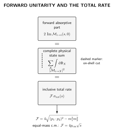
Unitarity matches the forward discontinuity to a convention-normalized sum over physical intermediate states. The diagram is schematic: Cutkosky rules provide a later diagram-by-diagram implementation, while the operator identity already requires a complete asymptotic-state basis.

Perturbative order counting

Expand $T=\sum_{n\ge1}g^nT^{(n)}$. At order $g^n$,

$$T^{(n)}-T^{(n)\dagger} =i\sum_{r=1}^{n-1}T^{(r)\dagger}T^{(n-r)}.$$

If a four-point tree amplitude begins at $g^2$, its one-loop imaginary part at $g^4$ is fixed by the phase-space integral of two tree amplitudes. A real tree amplitude below all propagator poles therefore does not violate unitarity; its absorptive part first appears when the perturbative right side has the corresponding order and an open intermediate channel.

For a concrete normalization check, take identical real scalars with $\mathcal L_{\mathrm{int}}=-\lambda\phi^4/4!$. Above $s=4m^2$, the two-scalar intermediate state contributes $1/2!$ and $\Phi_2=\rho/(8\pi)$, so at order $\lambda^2$ the forward relation gives

$$2\operatorname{Im}\mathcal M_{\text{1-loop}}(s,0) =\frac{1}{2!}\frac{\rho(s)}{8\pi}\lambda^2, \qquad \operatorname{Im}\mathcal M_{\text{1-loop}} =\frac{\lambda^2\rho(s)}{32\pi}.$$

This is the absorptive part of the physical $s$-channel bubble in the present normalization. Below threshold $\rho$ is not a physical phase-space factor and the state-sum contribution is zero; analytic continuation of the loop is a separate statement.

This order-by-order identity does not license selective resummation. Adding a width to one propagator while leaving other terms at tree order can spoil the same cancellations used to prove gauge identities. Generalized cuts and positivity bounds require additional structure: continue to generalized unitarity for cut-based reconstruction and to forward-limit positivity bounds only after the analytic and growth hypotheses are in place. The operator-level meaning of unitary time evolution remains with the foundational page linked above.

Check your understanding

Assume $T=gT^{(1)}+g^2T^{(2)}+\cdots$. Derive the anti-Hermitian part of $T^{(2)}$ and state which intermediate states are present. The check passes only if the complex conjugation reverses initial and final labels and the phase-space measure matches the state normalization.

Solution

The coefficient of $g^2$ in $T-T^\dagger=iT^\dagger T$ is

$$T^{(2)}-T^{(2)\dagger}=iT^{(1)\dagger}T^{(1)}.$$

Between states $f$ and $i$, insert the complete asymptotic identity to obtain $-i(\mathcal M^{(2)}_{fi}-\mathcal M^{(2)*}_{if})= \sum_X S_X^{-1}\int\mathrm d\Phi_X\, \mathcal M^{(1)*}_{Xf}\mathcal M^{(1)}_{Xi}$. The sum contains every kinematically open physical state reachable at first order, including its spin/species sums; $S_X^{-1}$ supplies its identical-particle factor. It is not restricted to the elastic channel unless all others are closed or excluded by exact quantum numbers.

References

• Schwartz, Matthew D. Quantum Field Theory and the Standard Model. Cambridge University Press, 2014, § 24.1, printed pp. 452–465. doi:10.1017/9781139540940.
• Weinberg, Steven. The Quantum Theory of Fields, Volume I: Foundations. Cambridge University Press, 1995, § 3.6, printed pp. 147–151. doi:10.1017/CBO9781139644167.