Collinear Factorization and Splitting Amplitudes

When two massless external momenta become parallel, an amplitude develops a universal pole associated with an almost on-shell parent. At leading power it factorizes into a lower-point amplitude and a splitting amplitude. The latter retains helicity and azimuthal information; only after squaring and averaging does it reduce to the familiar unpolarized splitting kernel.

Required background. Soft and Collinear Singularities identifies the collinear pinch and its overlap with a soft endpoint. Spinor-Helicity Variables supplies $\langle ab\rangle[ba]=s_{ab}$ and the helicity phases used below.

Collinear kinematics and the parent pole

Let $P$ and $n$ be null reference vectors with $P\cdot n>0$, and let $k_\perp$ be orthogonal to both. An exactly on-shell parameterization is

$$\begin{aligned} p_a^\mu &=zP^\mu+k_\perp^\mu -\frac{k_\perp^2}{z}\frac{n^\mu}{2P\cdot n},\\ p_b^\mu &=(1-z)P^\mu-k_\perp^\mu -\frac{k_\perp^2}{1-z}\frac{n^\mu}{2P\cdot n}, \end{aligned}$$

where $0<z<1$ for a final-state splitting and $k_\perp^2<0$. Direct substitution gives $p_a^2=p_b^2=0$ and

$$s_{ab}=(p_a+p_b)^2 =-\frac{k_\perp^2}{z(1-z)}\longrightarrow0.$$

Thus the actual parent momentum $p_{ab}=p_a+p_b$ approaches the null reference momentum $P$ with corrections of order $k_\perp^2$; the lower-point amplitude uses this on-shell projection. The invariant $s_{ab}$, not an arbitrary small spatial angle, is the covariant expansion parameter. The endpoints $z\to0$ or $1$ overlap with a soft limit and cannot be counted independently without a subtraction or a combined factorization formula.

The logarithmic energy-angle picture and representative momentum scalings are shown here for reference.

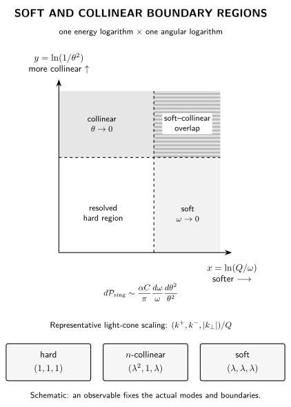
The collinear limit approaches the upper boundary at fixed energy fraction, whereas $z\to0$ or $1$ enters the soft-collinear overlap. The displayed regions and scalings are schematic; an observable determines the precise mode content and boundaries.

Amplitude-level factorization

For adjacent legs in a color-ordered tree amplitude, the leading limit is

$$\begin{aligned} &A_{n+1}^{\mathrm{tree}}(\ldots,a^{h_a},b^{h_b},\ldots) \xrightarrow[a\parallel b]{}\\ &\qquad\sum_{h=\pm} \operatorname{Split}^{\mathrm{tree}}_{-h} (a^{h_a},b^{h_b};z)\\ &\qquad\quad\times A_n^{\mathrm{tree}}(\ldots,P^h,\ldots). \end{aligned}$$

In this convention the gauge coupling and color generator are stripped from $A$ and from $\operatorname{Split}$. The splitting amplitude has mass dimension $-1$ and scales as $s_{ab}^{-1/2}$, so its square produces the $1/s_{ab}$ probability pole.

For example, the nonzero equal-positive-helicity gluon splitting is

$$\operatorname{Split}^{\mathrm{tree}}_{-}(a^+,b^+;z) =\frac{1}{\sqrt{z(1-z)}\,\langle ab\rangle},$$

while

$$\operatorname{Split}^{\mathrm{tree}}_{-}(a^-,b^-;z)=0.$$

Parity supplies the conjugate relations, and mixed-helicity splittings carry $z^2$ or $(1-z)^2$ weights. These formulas exhibit information that a scalar kernel cannot: a complex azimuthal phase, little-group weight, and a helicity-selection zero. Dixon derives the amplitude factorization and the complete $g\to gg$ helicity set in Dixon 1996, § 3.4, printed pp. 27–29, PDF.

For a full-color amplitude, the parent color index is contracted through the appropriate generator or structure constant. Nonadjacent legs in one color ordering do not have that ordering’s leading two-particle collinear pole, although the full color sum contains the physically allowed channels.

From splitting amplitudes to kernels

After summing unresolved colors and retaining the parent spin indices, the squared matrix element takes the operator form

$$\begin{aligned} |\mathcal M_{n+1}|^2 \xrightarrow[a\parallel b]{} {}&\frac{2g_s^2\mu^{2\epsilon}}{s_{ab}}\\ &\times\langle\mathcal M_n| \widehat P_{ab}(z,k_\perp;\epsilon) |\mathcal M_n\rangle. \end{aligned}$$

This normalization uses $d=4-2\epsilon$, a dimensionless coupling $\alpha_s=g_s^2/(4\pi)$, the dimensional-regularization scale $\mu$, and the conventional spin-correlated splitting operator. If the factor $\mu^\epsilon$ is instead absorbed into the $d$-dimensional coupling, it should not be inserted a second time. After averaging the parent spin and azimuth in four dimensions, the unregularized real-emission kernels include

$$\begin{aligned} P_{q\to qg}(z) &=C_F\frac{1+z^2}{1-z},\\ P_{g\to gg}(z) &=2C_A\left[ \frac{z}{1-z}+\frac{1-z}{z}\right.\\ &\qquad\left.+z(1-z)\right],\\ P_{g\to q\bar q}(z) &=T_R\left[z^2+(1-z)^2\right]. \end{aligned}$$

Here $z$ is the quark fraction in $q\to qg$, and one daughter fraction in the other channels. These are pointwise real-emission expressions: endpoint plus prescriptions, $\delta(1-z)$ terms, and $O(\epsilon)$ pieces arise only after virtual contributions, phase-space definitions, and a factorization scheme are specified. Catani and Grazzini state the all-parton collinear factorization in spin space in Catani and Grazzini 1999, § 2, printed pp. 2–5, PDF.

Squaring too early can therefore lose azimuthal spin correlations. A local subtraction term must reproduce the spin-correlated limit when the observable or phase-space map remains sensitive to it; a spin-averaged kernel is enough only after the corresponding average is justified.

Initial-state and multiparticle qualifications

Crossing a daughter to the initial state changes the allowed fraction range, the causal interpretation, color orientation, and phase-space Jacobian. In a hadronic calculation, the remaining initial-state collinear pole is absorbed into a parton distribution in a stated scheme and at a stated factorization scale. The final-state formula above is not a substitute for that step.

Three or more momenta can approach a common direction, and soft and collinear limits can be nested or simultaneous. Their leading behavior is again universal, but naive pairwise iteration can double count overlaps or miss correlated limits. Beyond tree level, splitting amplitudes themselves contain infrared poles and acquire loop-dependent phases. Universality fixes the singular residue; it does not make the complete finite amplitude universal.

Check your understanding

Use the Sudakov parameterization to verify $p_a^2=p_b^2=0$ and derive $s_{ab}=-k_\perp^2/[z(1-z)]$. Then square the displayed positive-helicity splitting amplitude and use $|\langle ab\rangle|^2=s_{ab}$ in real kinematics. Confirm the expected $1/[z(1-z)s_{ab}]$ singularity and identify both soft endpoints.

References

• Catani, Stefano, and Massimiliano Grazzini. “Collinear Factorization and Splitting Functions for Next-to-Next-to-Leading Order QCD Calculations.” Physics Letters B 446 (1999): 143–152, esp. § 2, printed pp. 2–5 of the author manuscript. doi:10.1016/S0370-2693(98)01513-5. Open PDF.
• Dixon, Lance J. “Calculating Scattering Amplitudes Efficiently.” In QCD and Beyond: Proceedings of TASI 1995, edited by David E. Soper, 539–582. World Scientific, 1996, esp. § 3.4, printed pp. 27–29 of the author manuscript. doi:10.1142/9789814503802_0006. Open PDF.