The Interaction Picture and Dyson Series

Splitting the Hamiltonian as $H=H_0+H_{\mathrm{int}}$ moves the exactly solvable evolution into the operators and leaves the state evolution generated by the interaction-picture Hamiltonian. Iterating that evolution equation gives integrals over ordered time simplices; equivalently, a factor $1/n!$ and the time-ordering operator extend each simplex to the full $n$-dimensional time domain. This is the Dyson series. It is a perturbative construction with a declared time interval, state prescription, regulator, and switching procedure—not a globally exact unitary equivalence between free and interacting relativistic fields.

Required background. Fock Space, Vacuum, and Particle Number supplies the free representation and the action of creation and annihilation operators used below.

Helpful background. Haag’s Theorem: Physical Meaning and Scope explains why the interaction picture requires a cutoff, finite-time use, or asymptotic interpretation; Interacting Fields, Asymptotic Observables, and Effective Descriptions separates that controlled use from a nonperturbative existence claim.

Interaction-picture evolution

Let $U(t,t_0)$ be the Schrödinger-picture evolution. For time-independent $H_0$, define the two-endpoint interaction-picture evolution consistently with the interaction-picture operators by

$$U_I(t,t_0) =e^{iH_0t}U(t,t_0)e^{-iH_0t_0}, \qquad \mathcal O_I(t)=e^{iH_0t}\mathcal O_S e^{-iH_0t}.$$

Then

$$i\frac{\partial}{\partial t}U_I(t,t_0) =H_I(t)U_I(t,t_0), \qquad H_I(t)=e^{iH_0t}H_{\mathrm{int}}e^{-iH_0t},$$

with $U_I(t_0,t_0)=1$. Integrating once gives the Volterra equation

$$U_I(t,t_0) =1-i\int_{t_0}^{t}\mathrm dt_1\, H_I(t_1)U_I(t_1,t_0).$$

The interaction-picture construction and this integral equation are derived in Weinberg 1995, § 3.5, pp. 142–143. Iteration, rather than an ordinary exponential, is necessary because $H_I(t_1)$ and $H_I(t_2)$ generally do not commute.

Ordered simplices and the Dyson series

Substituting the integral equation into itself produces

$$\begin{aligned} U_I(t,t_0) &=1-i\int_{t_0}^{t}\mathrm dt_1\,H_I(t_1)\\ &\quad+(-i)^2\int_{t_0}^{t}\mathrm dt_1 \int_{t_0}^{t_1}\mathrm dt_2\, H_I(t_1)H_I(t_2)+\cdots . \end{aligned}$$

At order $n$, the domain is the simplex

$$t\ge t_1\ge t_2\ge\cdots\ge t_n\ge t_0.$$

With a regulator that makes the operator products well defined and assigns no separate contact contribution to their coincidence sets, the $n!$ open simplices partition the hypercube $[t_0,t]^n$ up to their common boundaries. Time ordering places the latest operator to the left, so all $n!$ regions become copies of the same ordered integrand. If distributional contact terms occur, their prescription is part of the definition of the time-ordered product and cannot be discarded merely because it is supported at equal times. Under the regulated assumption just stated,

$$\boxed{ U_I(t,t_0) =\sum_{n=0}^{\infty}\frac{(-i)^n}{n!} \int_{t_0}^{t}\mathrm dt_1\cdots\mathrm dt_n\, \mathrm T\!\left[H_I(t_1)\cdots H_I(t_n)\right] }.$$

The notation $\mathrm T\exp[-i\int H_I]$ means precisely this series; it is not an instruction to ignore noncommutativity. Dyson’s original construction organizes the scattering operator by these ordered products Dyson 1949, pp. 1736–1743, while the simplex-to-hypercube step and its factorial are displayed explicitly in Weinberg 1995, § 3.5, pp. 143–144.

There is a useful sharp distinction between the finite-time operator theorem and its QFT use. If $H_I(t)$ is bounded and strongly measurable on $[t_0,t]$, with

$$K=\int_{t_0}^{t}\mathrm dt'\,\lVert H_I(t')\rVert<\infty,$$

then the norm of the $n$th ordered term is at most $K^n/n!$, so the series converges absolutely in operator norm. Unbounded Hamiltonians require a common invariant domain or a stronger evolution theorem. Local continuum interaction densities do not meet the bounded hypothesis without regulation, so their Dyson expansion is ordinarily interpreted coefficient by coefficient.

For a first field-theory application, take $\mathcal L_{\mathrm{int}}=-\lambda\phi_I^4/4!$, with no time derivatives. Only under that qualification may one use $\mathcal H_I=-\mathcal L_{\mathrm{int}}$, giving

$$H_I(t')=\frac{\lambda}{4!} \int\mathrm d^{d-1}\mathbf x\, \phi_I^4(t',\mathbf x),$$

and, writing $x_j=(t_j,\mathbf x_j)$,

$$\begin{aligned} U_I(t,t_0) &=1-\frac{i\lambda}{4!} \int_{t_0}^{t}\mathrm dt_1\int\mathrm d^{d-1}\mathbf x_1\, \phi_I^4(x_1)\\ &\quad+\frac{1}{2!}\left(\frac{-i\lambda}{4!}\right)^2 \int_{t_0}^{t}\mathrm dt_1\mathrm dt_2 \int\mathrm d^{d-1}\mathbf x_1\mathrm d^{d-1}\mathbf x_2\, \mathrm T\!\left[\phi_I^4(x_1)\phi_I^4(x_2)\right] +O(\lambda^3). \end{aligned}$$

The next page turns the labeled free fields in these ordered products into contractions; no graph or symmetry factor has yet been assumed here.

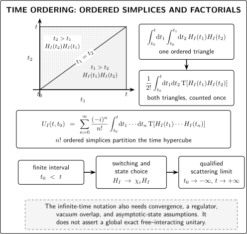
The figure encodes the same identity geometrically. Inspect the diagonal separating the two second-order orderings and the qualification attached to the infinite-time limit.

At second order, the regions $t_1>t_2$ and $t_2>t_1$ fill the time square and are mapped into one another by relabeling. Time ordering makes their operator products agree, producing the factor $1/2!$. Extending the endpoints to infinity is a separate, qualified scattering limit. Schematic, not to scale.

Representation	Domain	Operator order	Multiplicity
Iterated integral	$t_0<t_2<t_1<t$	$H_I(t_1)H_I(t_2)$	one ordered simplex
Complementary simplex	$t_0<t_1<t_2<t$	$H_I(t_2)H_I(t_1)$	obtained by exchanging labels
Time-ordered form	$(t_1,t_2)\in[t_0,t]^2$	later time always left	divide by $2!$
Scattering notation	endpoints formally sent to $\mp\infty$	same ordering	also requires asymptotic-state and convergence prescriptions

Checks and limiting cases

Commuting interaction. If $[H_I(t_1),H_I(t_2)]=0$ for all times, time ordering is inert and the series sums to the ordinary exponential

$$U_I(t,t_0)= \exp\!\left[-i\int_{t_0}^{t}\mathrm dt\,H_I(t)\right].$$

Composition. Uniqueness of the evolution equation gives

$$U_I(t_2,t_0)=U_I(t_2,t_1)U_I(t_1,t_0).$$

Expanding both sides through second order partitions the ordered simplex according to whether both insertions lie before $t_1$, both after it, or one on each side.

Unitarity. For Hermitian $H_I$, the adjoint equation implies $\partial_t(U_I^\dagger U_I)=0$. At second order, the two time orderings in $U_I^{(2)}+U_I^{(2)\dagger}$ cancel the product $U_I^{(1)\dagger}U_I^{(1)}$. A truncation is unitary only up to terms beyond the retained order.

Noncommuting pulses. Let $H_I=A$ for $0<t<\Delta$ and $H_I=B$ for $\Delta<t<2\Delta$, with $[A,B]\ne0$. Composition gives

$$U_I(2\Delta,0)=e^{-iB\Delta}e^{-iA\Delta} =1-i\Delta(A+B)-\frac{\Delta^2}{2}(A^2+B^2)-\Delta^2BA+O(\Delta^3).$$

The mixed product is $BA$, because the later pulse stands to the left. The ordinary exponential $e^{-i\Delta(A+B)}$ instead averages $AB$ and $BA$; their difference starts at $\Delta^2[A,B]/2$. This checks both the operator order and the need for $\mathrm T$.

Switching, vacuum selection, and Haag’s theorem

For scattering one often makes the replacement $H_I(t)\mapsto\chi_\epsilon(t)H_I(t)$, with $\chi_\epsilon$ tending to zero at large $|t|$, and only afterward studies a limit such as $\epsilon\to0^+$. A convergence factor also fixes the boundary value that becomes the Feynman $+i0$ prescription and may project onto the desired vacuum when overlap and spectral assumptions hold. Weinberg makes the convergence factor explicit in the passage from energy denominators to time integrals Weinberg 1995, § 3.5, p. 143.

These devices do not prove that the interacting Hilbert-space representation is unitarily equivalent to the free Fock representation. In infinite-volume relativistic QFT, Haag’s theorem obstructs that literal global reading under its hypotheses. Perturbation theory remains meaningful with regulators, finite-time evolution, finite volume, renormalized asymptotic constructions, or formal power-series interpretation, but the chosen meaning must be stated. Nor is convergence in the coupling guaranteed: the Dyson series is normally used order by order, with its truncation and regulator dependence kept visible.

Common pitfalls

Dropping time ordering inside an exponential. The compact exponential is notation for the ordered series. It becomes an ordinary exponential only under a commutativity condition.

Treating adiabatic switching as a theorem about physical preparation. Switching is a calculational prescription whose removal can fail, especially in theories with massless long-range interactions or without suitable asymptotic states.

Claiming exact free–interacting equivalence. Interaction-picture fields are the free fields used inside a regulated or asymptotic perturbative construction. Their usefulness does not supply a global intertwining unitary for the exact theory.

Check your understanding

Expand $U_I(t_2,t_0)$ to second order and divide its ordered domain at an intermediate time $t_1$. Show explicitly that the result equals $U_I(t_2,t_1)U_I(t_1,t_0)$ through the same order.

Solution

Split the ordered region $t_2>\tau_1>\tau_2>t_0$ into three disjoint pieces: both times above $t_1$, both below it, and $\tau_1>t_1>\tau_2$. The first two pieces are the second-order terms of $U_I(t_2,t_1)$ and $U_I(t_1,t_0)$. The mixed piece factorizes as

$$(-i)^2\int_{t_1}^{t_2}\mathrm d\tau_1\,H_I(\tau_1) \int_{t_0}^{t_1}\mathrm d\tau_2\,H_I(\tau_2),$$

which is the product of their first-order terms, with the later operator already on the left. Together with the zeroth- and first-order pieces this is precisely the expansion of $U_I(t_2,t_1)U_I(t_1,t_0)$.

Where to continue

• Turn ordered products into contractions: Wick Expansion for Interacting Fields applies the free-field theorem inside the Dyson numerator and denominator.
• Check the representation-theoretic limitation: Haag’s Theorem: Physical Meaning and Scope states the hypotheses behind the obstruction.
• Proceed toward observables after the rule set is complete: Asymptotic States, LSZ, and Scattering Observables explains what additional pole and asymptotic-state assumptions convert correlators into scattering amplitudes.

References

• Dyson, Freeman J. “The S Matrix in Quantum Electrodynamics.” Physical Review 75, no. 11 (1949): 1736–1755. DOI.
• Weinberg, Steven. The Quantum Theory of Fields, Volume I: Foundations. Cambridge: Cambridge University Press, 1995. First edition; 2005 paperback, 2012 printing consulted. DOI.