Leading Singularities and Integrand Geometry

A leading singularity is a maximal multidimensional residue of a loop integrand, evaluated on a contour that surrounds enough on-shell hypersurfaces to localize all remaining integration variables. It captures local numerator, Jacobian, and factorization data. It is not the same object as a branch point of the integrated amplitude, and its sign and normalization depend on contour orientation.

Required background. Generalized Unitarity and Integrand Reduction supplies maximal cuts and integrand equivalence, while Laurent Series, Poles, and Residues supplies the one-variable residue concept generalized below.

Multidimensional residues

Near an isolated common zero $z_*$ of $n$ denominators, write the meromorphic $n$-form

$$\Omega(z)= \frac{N(z)\,\mathrm dz_1\wedge\cdots\wedge\mathrm dz_n} {D_1(z)\cdots D_n(z)}.$$

If the Jacobian is nonzero,

$$\det\!\left(\frac{\partial D_i}{\partial z_j}\right)_{z_*}\ne0,$$

then the ordered small torus

$$\Gamma_{\boldsymbol\varepsilon} =\{z:|D_i(z)|=\varepsilon_i,\ i=1,\ldots,n\},$$

oriented by $\mathrm d\arg D_1\wedge\cdots\wedge\mathrm d\arg D_n>0$, fixes the normalization

$$\begin{aligned} \operatorname{Res}_{z_*}\Omega &:=\frac{1}{(2\pi i)^n} \int_{\Gamma_{\boldsymbol\varepsilon}}\Omega \\ &=\frac{N(z_*)} {\det(\partial D_i/\partial z_j)_{z_*}}. \end{aligned}$$

Permuting two ordered denominators or reversing one circle reverses the sign. A zero of $N$ can cancel the candidate pole; a degenerate Jacobian requires a more careful local residue rather than this simple formula.

At one loop in four dimensions a generic quadruple cut supplies four equations for four complex variables. At higher loops the count depends on the chosen variables, irreducible scalar products, and pole structure; “cut every propagator” need not fully localize the form.

For a concrete massless scalar box, take

$$p_1=Q(-1,0,0,-1),\quad p_2=Q(-1,0,0,1),\quad p_3=Q(1,1,0,0),\quad p_4=Q(1,-1,0,0),$$

and denominators $\rho_1=\ell^2$, $\rho_2=(\ell+p_1)^2$, $\rho_3=(\ell+p_1+p_2)^2$, $\rho_4=(\ell-p_4)^2$. The cut equations have two solutions

$$\ell_\pm=Q(1,-1,\pm i,1).$$

For the ordered measure $\mathrm d\ell^0\wedge\mathrm d\ell^1\wedge\mathrm d\ell^2\wedge\mathrm d\ell^3$ and contour order $(\rho_1,\rho_2,\rho_3,\rho_4)$, the Jacobians are $J_\pm=\mp32iQ^4$. Hence the form $g^4\mathrm d^4\ell/(\rho_1\rho_2\rho_3\rho_4)$ has

$$\operatorname{LS}_\pm =\frac{g^4}{J_\pm} =\pm\frac{i g^4}{32Q^4}.$$

The pole-stripped tree-sewn values are instead $R_\pm=J_\pm\operatorname{LS}_\pm=g^4$. Thus the two oriented residues cancel if added without weights, while the scalar-box coefficient is their basis-normalized tree datum. This example makes orientation, solution summation, and Jacobian normalization separate operations rather than a single “maximal cut.”

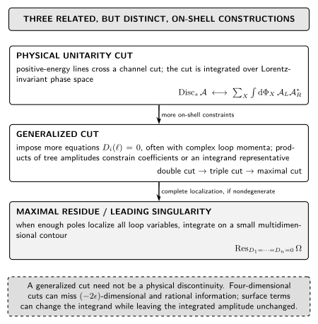
Leading singularities are oriented local residues when the cut equations completely and nondegenerately localize the loop form. The diagram is schematic and not to scale; degeneracies, doubled propagators, poles at infinity, and dimensionally hidden terms require separate analysis.

dlog forms and constant residues

If a form can be written locally as

$$\Omega=C\, \mathrm d\log f_1\wedge\cdots\wedge\mathrm d\log f_n,$$

then its simple maximal residues are $\pm C$ for compatible orientations. Constant leading singularities often suggest a normalization in which a master integral has uniform transcendental behavior and a simple differential equation. This is a powerful basis-selection heuristic, not an equivalence valid for every integral family.

The relation among maximal cuts, leading singularities, and canonical $\mathrm d\log$ bases—together with its conjectural limits—is reviewed in Abreu, Britto, and Duhr 2022, §3.3.2, p. 34. A constructive multiloop discussion appears in Weinzierl 2022, §7.1.7, pp. 268–272.

What the residue does and does not establish

A maximal cut factorizes into trees only after the internal state sum, solution set, and dimensional scheme are specified. Constancy of a residue follows from an explicit numerator and Jacobian calculation, with contour orientation and all isolated solutions retained. A local $\mathrm d\log$ form establishes simple logarithmic poles in that chart, but not the absence of poles at infinity or the existence of compatible global charts. Unit leading singularities can motivate a canonical basis; the full differential system and boundary data must still confirm it.

Most importantly, a leading singularity alone does not establish a physical branch cut of the integrated amplitude. That claim additionally needs a Landau pinch, a sheet and energy-flow assignment, and the actual integration contour. The shared evidence-status table places leading-singularity and geometric statements beside their theory domain, support, limitations, and unresolved implications.

These distinctions prevent three common overclaims. First, an integrand pole may integrate to zero or be canceled in the amplitude. Second, an integrated branch point can arise from an extended pinch rather than an isolated maximal residue. Third, two surface-term-related integrands may have different local presentations even though their regulated integrals agree.

Numerators, poles at infinity, and geometry

Choosing a numerator changes residues without changing the denominator graph. A well-chosen numerator can cancel unwanted poles, normalize all nonzero leading singularities, or improve behavior at infinity. Conversely, a numerator can introduce higher-degree growth and reveal a pole at the compactification boundary.

Geometric language is useful when boundaries of a parameter or momentum-space region correspond to logarithmic poles and their iterated intersections. But a claimed geometry must specify its variables, differential form, contour, orientation, and theory. A suggestive polytope or $\mathrm d\log$ expression is not by itself a proof that the integrated QFT amplitude is a canonical form of that geometry.

A two-variable check

For

$$\Omega=C\,\frac{\mathrm dz_1\wedge\mathrm dz_2}{z_1z_2},$$

take both circles counterclockwise in the ordered contour $(z_1,z_2)$. Then

$$\frac{1}{(2\pi i)^2}\oint_{|z_1|=\varepsilon_1} \oint_{|z_2|=\varepsilon_2}\Omega=C.$$

Exchanging the wedge order gives $-C$. This elementary calculation is the normalization model for a maximal residue after using $D_i$ as local coordinates.

Exercises

1. What happens if $N(z_*)=0$ in the simple-residue formula? The maximal residue vanishes even though the denominator equations have a common solution.
2. Why does a unit leading singularity not determine an integrated master? It fixes local residue normalization, not boundary constants, lower-codimension cuts, or the continuation path.

Where residue geometry is tested

• Differential Equations for Master Integrals tests whether a residue-motivated normalization actually produces a simple differential system with consistent boundary data.
• Color–Kinematics Duality places geometric integrand claims in a theory-specific comparison of evidence, limitations, and unresolved extensions.

References

• Abreu, Samuel, Ruth Britto, and Claude Duhr. “The SAGEX Review on Scattering Amplitudes, Chapter 3: Mathematical Structures in Feynman Integrals.” Journal of Physics A: Mathematical and Theoretical 55 (2022): 443004, 56 pp. doi:10.1088/1751-8121/ac87de. Open PDF.
• Weinzierl, Stefan. Feynman Integrals: A Comprehensive Treatment for Students and Researchers. Cham: Springer, 2022. doi:10.1007/978-3-030-99558-4. Open prepublication PDF.