Hard, Jet, and Soft Factorization

A hard–jet–soft formula is justified when an observable has a short-distance scale, energetic nearly collinear directions, and low-energy radiation whose leading interactions can be separated without double counting. The result is not a universal product attached to every process: its functions, convolutions, Wilson-line geometry, regulators, and power corrections are defined by a specific observable and a process-specific factorization argument.

Required background. Collinear Factorization and Splitting Amplitudes supplies the universal collinear limit. Eikonal Approximation and Wilson Lines supplies the soft color sources and their causal orientation.

Helpful background. Bloch–Nordsieck and KLN Cancellation explains why an infrared- safe measurement is needed before separated real and virtual sectors can combine into a finite observable.

A representative factorization formula

Consider the two-jet limit of $e^+e^-$ annihilation and let $\tau=1-T\ll1$ be thrust, with

$$T=\max_{\widehat{\boldsymbol t}} \frac{\sum_j|\widehat{\boldsymbol t}\cdot\boldsymbol p_j|} {\sum_j|\boldsymbol p_j|}.$$

If $s_n$ and $s_{\bar n}$ are the collinear hemisphere invariant masses and $k$ is the dimension-one soft contribution, the leading measurement is

$$\tau=\frac{s_n+s_{\bar n}}{Q^2}+\frac{k}{Q}+O(\tau^2).$$

At leading power, a standard schematic formula is

$$\begin{aligned} \frac{1}{\sigma_0}\frac{\mathrm d\sigma}{\mathrm d\tau} ={}&H(Q^2,\mu)\\ &\times\int \mathrm ds_n\,\mathrm ds_{\bar n}\,\mathrm dk\\ &\times J_n(s_n,\mu)J_{\bar n}(s_{\bar n},\mu)\\ &\times S(k,\mu)\\ &\times\delta\!\Bigg( \tau-\frac{s_n+s_{\bar n}}{Q^2}\\ &\qquad\qquad-\frac{k}{Q}\Bigg)+O(\tau). \end{aligned}$$

The terms have distinct jobs:

• $H$ is the squared short-distance matching coefficient at virtuality $Q^2$.
• $J_n$ and $J_{\bar n}$ describe collinear radiation and invariant masses in the two energetic directions.
• $S$ is a vacuum matrix element of appropriately oriented soft Wilson lines with the soft part of the thrust measurement inserted.
• The delta function is not decorative: it states how sector momenta combine into the measured value.

The omitted $O(\tau)$ terms include subleading operators, recoil and measurement corrections. Nonperturbative corrections become important when the lowest dynamical scale approaches $\Lambda_{\mathrm{QCD}}$. Schwartz derives the two-jet effective-theory separation and thrust measurement in Schwartz 2014, §§ 36.2–36.5, printed pp. 780–802.

Two normalization checks are immediate. In the convention displayed above,

$$[H]=0, \qquad [J(s)]=-2, \qquad [S(k)]=-1,$$

so the three integrations cancel the dimensions of the two jet functions and the soft function. At tree level,

$$H^{(0)}=1, \qquad J^{(0)}(s)=\delta(s), \qquad S^{(0)}(k)=\delta(k),$$

and the convolution returns $\delta(\tau)$. A formula that misses either check has not implemented the measurement normalization correctly.

Natural scales and common evolution

For small thrust, fixed-order logarithms are minimized near

$$\mu_H\sim Q, \qquad \mu_J\sim Q\sqrt{\tau}, \qquad \mu_S\sim Q\tau.$$

Each function is computed near its natural scale and evolved to a common renormalization scale $\mu$. The combined cross section must be independent of that arbitrary common scale up to the perturbative and power accuracy retained. In convolution notation this requires the anomalous dimensions to cancel,

$$\gamma_H+\gamma_{J_n}+\gamma_{J_{\bar n}}+\gamma_S=0,$$

with products interpreted as kernels where the measured variable is convolved. This consistency relation is a powerful check, but satisfying it does not by itself prove that no leading region is missing.

The scale flow and its connection to fixed-order matching are summarized below. Inspect the two qualifications at the bottom: overlap subtraction is part of the definition, and rapidity or Glauber effects may require more than ordinary $\mu$ evolution.

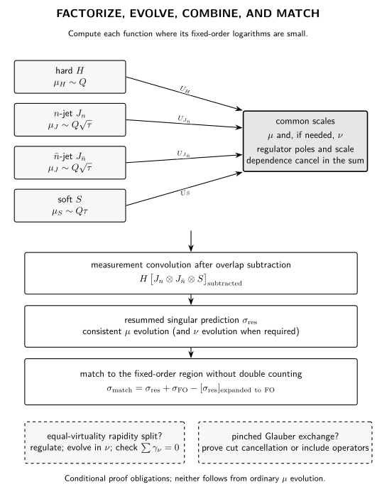
Scale separation for a representative dijet observable. Hard, jet, and soft functions are computed near $Q$, $Q\sqrt\tau$, and $Q\tau$, evolved consistently, combined with overlap subtraction, and matched to the fixed- order region. A rapidity scale $\nu$ or a Glauber analysis is needed only when the corresponding regions occur. The diagram is schematic and not to scale.

Overlap subtraction is part of the definition

The soft expansion extends into the zero-momentum boundary of each collinear sector, while a collinear loop can reproduce the same limiting integrand. Adding sector integrals without subtracting that overlap double counts a leading region. In one common effective-theory organization the collinear “zero-bin” is subtracted; in other organizations a soft division or an equivalent region subtraction performs the same bookkeeping. Individual functions can therefore differ between schemes even when the physical convolution agrees.

Dimensional regularization and $\overline{\mathrm{MS}}$ are a frequent local choice, not part of the physical theorem. Scaleless overlap terms may vanish as integrals in pure dimensional regularization while still carrying the UV–IR assignment needed for anomalous dimensions. If soft and collinear modes have equal invariant mass but different rapidities, dimensional regularization does not regulate their separation and a rapidity regulator, rapidity scale $\nu$, and corresponding subtraction are required.

Becher, Broggio, and Ferroglia develop matching, soft decoupling, jet and soft functions, and renormalization-group consistency in their SCET introduction, arXiv PDF §§ 4.5–7, printed pp. 38–90.

What a factorization argument must establish

A credible leading-power formula must do more than name three functions. It must:

1. identify every leading pinch surface and its momentum scaling;
2. show that hard, collinear, and soft approximations reproduce those regions;
3. use Ward identities to move leading soft couplings onto Wilson lines;
4. define the measurement in each sector and the convolution that recombines it;
5. subtract overlaps and demonstrate regulator cancellation;
6. prove cancellation or controlled inclusion of Glauber exchange;
7. state the power expansion, factorization and rapidity schemes, and nonperturbative domain.

Collins, Soper, and Sterman explain this pinch-surface, approximation, Ward- identity, and remainder logic for hard QCD processes in Collins, Soper, and Sterman 2004, §§ 8–9, printed pp. 76–95, PDF.

Universality is correspondingly qualified. A jet function can recur across observables with the same collinear operator and measurement, and a soft function can recur with the same Wilson-line directions, representations, and measurement. Changing any of those data can change the function. Parton distributions, transverse-momentum factorization, non-global measurements, and process-specific Glauber cancellation require their own statements.

Check your understanding

Check the thrust formula dimensionally: $s_n$ and $s_{\bar n}$ have dimension two, $k$ has dimension one, and every term in the delta-function argument is dimensionless. Then set $\tau=10^{-2}$ and order the three natural scales. Explain why evaluating every function at $Q$ leaves large logarithms even though the final cross section is formally independent of $\mu$.

References

• Becher, Thomas, Alessandro Broggio, and Andrea Ferroglia. Introduction to Soft-Collinear Effective Theory. Lecture Notes in Physics 896. Springer, 2015, §§ 4.5–7. doi:10.1007/978-3-319-14848-9. Open PDF.
• Collins, John C., Davison E. Soper, and George Sterman. “Factorization of Hard Processes in QCD.” In Perturbative Quantum Chromodynamics, edited by A. H. Mueller, 1–91. World Scientific, 1989; updated author manuscript, 2004, §§ 8–9, printed pp. 76–95. doi:10.1142/9789814503266_0001. Open PDF.
• Schwartz, Matthew D. Quantum Field Theory and the Standard Model. Cambridge University Press, 2014, §§ 36.2–36.5, printed pp. 780–802. doi:10.1017/9781139540940.