One-Loop Integral Families and Analytic Functions

At one loop, the basic one- through four-denominator scalar integrals form the tadpole, bubble, triangle, and box families. Pentagon and higher-point families also occur; in generic four-dimensional kinematics they can be reduced to lower-point integrals, while dimension-dependent remainders and Gram-degenerate limits require care. Weinzierl 2022, §5.2, pp. 141–143 gives the reduction through $O(\epsilon^0)$ and shows where higher-order remainders enter. Topology does not by itself determine the answer: internal masses, external virtualities, numerator powers, dimension, and boundary prescription select the scales and branch loci. The basic families generate algebraic functions, logarithms, and dilogarithms.

Required background. Dimensional Regularization as an Amplitude Tool supplies the $d=4-2\epsilon$ continuation and normalization of the scalar loop integral.

Helpful background. Branches, Sheets, Continuation, and Monodromy supplies the complex-analysis language needed to continue logarithms and polylogarithms across thresholds.

The scalar N-point family

Write a one-loop scalar integral as

$$I_N^{(d)}(\nu_1,\ldots,\nu_N) =\mu^{2\epsilon}\int\frac{\mathrm d^d\ell}{(2\pi)^d} \prod_{j=1}^{N}\frac{1}{[(\ell+P_j)^2-m_j^2+i0]^{\nu_j}}.$$

Shifts of all $P_j$ by the same vector are routing changes; only their differences are physical. Pinching a denominator, $\nu_j=0$, moves to a lower-point sector. If the numerator is independent of $m_j^2$, this denominator convention gives the exact relation

$$\frac{\partial}{\partial m_j^2}I_N^{(d)}(\ldots,\nu_j,\ldots) =\nu_j I_N^{(d)}(\ldots,\nu_j+1,\ldots),$$

understood first in a convergence domain and then by analytic continuation.

The useful map is summarized below and in the figure.

Family	Independent denominator data	Generic function content near four dimensions	First analytic feature to inspect
Tadpole	one mass	powers and logarithms	UV pole; no external channel
Bubble	one invariant, two masses	logarithms and a square root	two-particle threshold
Triangle	three external virtualities, three masses	logarithms and dilogarithms	normal and possible anomalous thresholds
Box	several invariants and four masses	dilogarithms in generic one-loop cases	intersecting channel branch surfaces

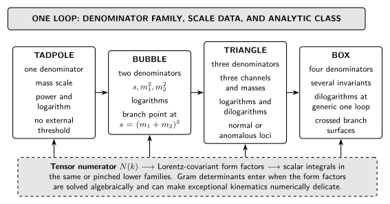
The map shows the basic one- through four-point sector and separates denominator topology from its scale and branch data; it is not an exhaustive list of higher-point one-loop families. It is schematic and not to scale: special masses or kinematics can simplify a family, while Gram-degenerate points require a representation adapted to the limit.

Passarino–Veltman reduction and the basic one-loop scalar set are developed in Weinzierl 2022, §§5.1–5.3, pp. 138–146.

Tadpole and bubble

With the normalization of the dimensional-regularization page, the tadpole is

$$T(m^2)=\mu^{2\epsilon}\int\frac{\mathrm d^d\ell}{(2\pi)^d} \frac{1}{\ell^2-m^2+i0} =-\frac{i}{(4\pi)^{d/2}} \Gamma\!\left(1-\frac d2\right) \mu^{2\epsilon}(m^2-i0)^{d/2-1}.$$

Its mass dimension is two. A massless tadpole is scaleless and vanishes in dimensional regularization; this is not the same as a finite massive tadpole at $m\to0$ term by term.

For the equal-mass bubble it is useful to subtract at $s=0$, eliminating its UV constant:

$$\widehat B(s;m^2) =B(s;m^2)-B(0;m^2) =-\frac{i}{(4\pi)^2} \int_0^1\mathrm d x\, \log\!\left[1-\frac{s}{m^2}x(1-x)-i0\right] +O(\epsilon).$$

Below $s=4m^2$ the bracket is positive and the finite function is real apart from the displayed overall loop convention. Above threshold, it is negative on an interval between the two roots. The square root

$$\beta(s)=\sqrt{1-\frac{4m^2}{s+i0}}$$

measures the length of that interval and controls the discontinuity. The square root is continued from the upper half of the $s$ plane and is positive for real $s>4m^2$. The $-i0$ fixes the logarithm below its negative-real-axis cut. This simple parameter integral is often safer than memorizing a closed form whose logarithm convention is unstated.

For the dimensionless finite function $F(s)=(4\pi)^2\widehat B(s)/i$, the physical-sheet result is

$$F(s)= \begin{cases} 2-2\rho\arctan(1/\rho),&0<s<4m^2,\\[3pt] 2-\beta\log\dfrac{1+\beta}{1-\beta}+i\pi\beta,&s>4m^2, \end{cases}$$

where $\rho=\sqrt{4m^2/s-1}$ and $\beta=\sqrt{1-4m^2/s}$. Thus $F(m^2)=2-\pi/\sqrt3$ is real, while $\operatorname{Im}F(5m^2)=\pi/\sqrt5$. These values independently test the Euclidean anchor, threshold location, and sign of the $-i0$ continuation.

Why triangles and boxes produce dilogarithms

After loop integration, a one-loop $N$-point function is a projective parameter integral with a quadratic kinematic polynomial. One parameter integration generally produces a logarithm. A second integration of the form

$$\int\frac{\mathrm d x}{x-a}\log(1-bx)$$

produces a dilogarithm. Thus triangles and boxes naturally generate $\operatorname{Li}_2$ functions, together with algebraic square roots and logarithms. This is a structural statement, not a claim that every special case needs a dilogarithm: massless or symmetric limits can collapse to logarithms, and singular limits can require distributions or an expansion in $\epsilon$.

Explicit massless scalar one-loop formulas and their continuation are collected in Weinzierl 2022, Appendix B, pp. 575–580.

Branch and normalization checks

Three checks catch many one-loop mistakes:

1. Dimension. With unit propagator powers, $I_N^{(4)}$ has mass dimension $4-2N$ before numerator factors; for general powers it is $4-2\sum_j\nu_j$.
2. Conjugation. With real masses and invariants away from cuts, reversing $i0$ complex-conjugates the scalar boundary value.
3. Threshold. The equal-mass bubble has no physical two-particle discontinuity below $4m^2$, and its phase-space factor vanishes as $\beta\to0^+$.

The topology alone cannot fix a branch. Always continue from a Euclidean point or state an equivalent prescription.

Exercises

1. Differentiate $T(m^2)$ with respect to $m^2$. The result is the one-denominator integral with power two, with a positive sign because $d(\ell^2-m^2)^{-1}/d m^2=(\ell^2-m^2)^{-2}$.
2. Find where the bubble logarithm first reaches its cut. Since $x(1-x)\le1/4$, this occurs at $s=4m^2$ and $x=1/2$.

Where the one-loop families lead

• Tensor Reduction expresses loop-momentum numerators through these scalar families and identifies Gram-sensitive limits.
• Landau Equations and Physical Singularities determines which denominator configurations can generate the branch loci seen in the scalar functions.

References

• Weinzierl, Stefan. Feynman Integrals. Cham: Springer, 2022. doi:10.1007/978-3-030-99558-4. Open PDF.