

Gauge-Fixed Perturbation Rules, Ghost Diagrams, and Identity Checks
Gauge-fixed perturbation theory starts from a declared gauge-fixed action, not from the gauge-invariant quadratic form alone. The gauge-fixing term makes the gauge-field kernel invertible, the Faddeev–Popov determinant becomes an action for Grassmann-odd ghosts, and ordinary action-to-rule translation then yields gauge, ghost, matter, and—when the symmetry is broken—Goldstone ingredients. These ingredients depend on the gauge parameter; consistency is tested only after assembling the complete amplitude or Green-function identity required by Ward or Slavnov–Taylor structure.
Required background. Momentum-Space Feynman Rules supplies kernel inversion and vertex translation; The Faddeev–Popov Construction supplies the determinant; Ghosts, Auxiliary Fields, and Gauge-Parameter Dependence fixes the ghost and gauge-parameter meaning imported here.
Helpful background. BRST Cohomology and Physical Observables identifies the physical sector; Slavnov–Taylor and Zinn-Justin Identities develops the general identities; Covariant Free-Photon Quantization and Propagator provides the Abelian propagator check.
A declared covariant gauge-fixed action
Section titled “A declared covariant gauge-fixed action”Take a compact gauge algebra with Hermitian generators and
For the linear covariant gauge , use
The ghost fields are independent Grassmann-odd Lorentz scalars in the adjoint representation. Integrating the second term by parts gives
up to a boundary term. This form fixes which momentum appears in the ghost vertex. The original Faddeev–Popov construction introduces the determinant precisely to correct gauge-orbit overcounting in perturbative diagrams Faddeev and Popov 1967, pp. 29–30. A detailed path-integral translation in compatible but not identical sign conventions appears in Srednicki 2007, §§ 71–72, pp. 420–426.
This page assumes that construction. It does not claim that the gauge condition supplies one representative on every gauge orbit.
Propagators and the ghost–gauge vertex
Section titled “Propagators and the ghost–gauge vertex”Introduce the transverse and longitudinal projectors for ,
If an term is added to the quadratic kernel before inversion, its transverse and longitudinal eigenvalues are regulated differently. The exact finite- inverse is
Consequently,
at finite regulator. For fixed , the boundary value is conventionally written
The in the longitudinal projector is understood through the regulated projector expression above. Replacing it by another does not give the inverse of the finite- kernel or obey the displayed contraction identity. At the two eigenspaces combine into Feynman gauge, while the boundary value is Landau gauge.
The free ghost rule is
With all momenta incoming, let be the momentum on the differentiated antighost field in the integrated-by-parts action. The ghost–antighost–gauge vertex is then
If the ghost arrow or integration-by-parts convention is reversed, the displayed momentum and sign change together. A valid translation changes both, then checks a complete amplitude. Every closed ghost loop carries an additional because the ghosts are Grassmann odd, even though they have no spinor index.
The Yang–Mills term supplies the three- and four-gauge vertices. Its cubic part is
With , the factor from , and all six assignments of the three labeled gauge fields included, three incoming momenta give
The overall sign and momentum differences agree with the action-level derivation in Srednicki 2007, § 72, p. 424, Eq. (72.5).
Contracting the first leg provides an action-level sign check. With ,
Thus the longitudinal contraction becomes a difference of inverse transverse kernels. In a complete non-Abelian Green-function identity, gauge-fixing and ghost terms extend this elementary relation to the Slavnov–Taylor statement.
The four-gauge vertex follows by differentiating the quartic part of and is proportional to times the three pairings of two structure constants and two metrics. Deriving it from the action is safer than importing a catalog whose generator, , or momentum convention may differ.
From gauge fixing to a physical check
Section titled “From gauge fixing to a physical check”The diagram below separates the three logical stages: declare the gauge-fixed action, read its gauge and ghost ingredients, and test only a complete object.
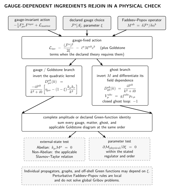
Gauge fixing makes the quadratic kernel invertible and the Faddeev–Popov operator supplies Grassmann-odd ghost propagators and vertices. Neither branch is physical by itself. The branches rejoin only in a complete amplitude or Green-function identity, where longitudinal and gauge-parameter dependence are tested. Schematic, not to scale.
| Stage | Input | Output | Check |
|---|---|---|---|
| gauge fixing | invertible | at finite regulator, | |
| Faddeev–Popov operator | ghost propagator and vertex | Abelian makes the determinant field independent | |
| graph assembly | gauge, matter, ghost, and applicable Goldstone diagrams | gauge-dependent intermediate amplitude | preserve all relative signs and symmetry factors |
| identity test | complete external-state or Green-function object | Ward or Slavnov–Taylor relation | unphysical polarizations and dependence cancel in the stated physical quantity |
Abelian and non-Abelian checks
Section titled “Abelian and non-Abelian checks”Abelian decoupling. For , the Faddeev–Popov operator in a linear covariant gauge is field independent. Its determinant is a source-independent normalization, so no interacting ghost diagram occurs. This reproduces covariant QED.
External photon Ward check. For an on-shell amplitude with one external photon and all required diagrams included,
under the usual physical-state and current-conservation assumptions. Replacing a physical polarization by its momentum must annihilate the sum, not necessarily each graph.
Non-Abelian identity check. In Yang–Mills theory, contracting a gauge leg generally relates several Green functions and includes ghost contributions. The correct statement is a Slavnov–Taylor identity following from BRST symmetry, not a diagram-by-diagram copy of the Abelian Ward identity. Taylor’s all-orders analysis makes the ghost-dependent structure explicit Taylor 1971, pp. 436–444, and Slavnov’s functional identities organize the corresponding gauge-theory relations Slavnov 1972, pp. 99–107.
Gauge-parameter check. A physical on-shell amplitude between BRST-closed states must be independent of when all contributions at the stated order are included and the regularization and renormalization preserve the identity. An individual propagator, self-energy component, or off-shell Green function may depend on .
Broken gauges and Goldstone fields
Section titled “Broken gauges and Goldstone fields”If the declared theory is spontaneously broken, a common gauge uses
where are the applicable Goldstone fields and is fixed by the vacuum and representation. The gauge-fixing term cancels gauge–Goldstone mixing, while the Faddeev–Popov operator can give ghosts a gauge-dependent mass and additional scalar couplings. The quadratic action must be diagonalized before propagators are quoted.
No universal vertex catalog follows from this schematic formula: the scalar representation, vacuum, generator normalization, and gauge-fixing function determine the tensors. Gauge Theories and the Standard Model provides those model-specific rules. The invariant checks remain the same—correct pole structure, cancellation of mixing, Slavnov–Taylor identities, and gauge-parameter independence of physical observables.
Perturbative scope and the Gribov limitation
Section titled “Perturbative scope and the Gribov limitation”The Faddeev–Popov construction is a local perturbative coordinate choice near a suitable background. Globally, a gauge condition can intersect an orbit more than once or develop zero modes of the Faddeev–Popov operator. These Gribov phenomena are not repaired by adding ordinary ghost diagrams, and this page makes no claim that they are. Conversely, the existence of a global issue does not invalidate the local weak-field rules in their controlled domain.
Ghosts are not asymptotic particles. They are bookkeeping fields whose loops enforce the identities needed to cancel unphysical gauge modes. Cutting or interpreting a ghost line as a detector state is outside the physical state space.
Common pitfalls
Section titled “Common pitfalls”Calling the gauge propagator an observable. Its longitudinal part and pole presentation depend on . Only a properly defined physical quantity is required to be gauge-parameter independent.
Omitting ghost loops because ghosts are unphysical. In a non-Abelian covariant gauge, the ghost determinant is field dependent. Ghost diagrams are required precisely so unphysical gauge contributions cancel consistently.
Testing one graph with a Ward identity. Gauge identities constrain the complete set of diagrams and, in non-Abelian theories, relate gauge and ghost Green functions.
Claiming perturbative gauge fixing is global. A nonzero local Faddeev–Popov determinant does not prove one representative per orbit over the full configuration space.
Check your understanding
Section titled “Check your understanding”Set in the declared action. Show what happens to the ghosts, contract the regulated photon propagator, and state where the on-shell Ward check applies.
Solution
When , , so the Faddeev–Popov operator is independent of . Its determinant is a source-independent normalization and the vertex vanishes. The projector formula gives
which becomes the standard boundary value. Finally, tests the sum of all diagrams for the complete on-shell amplitude with a conserved external current; it is not required graph by graph or for a generic off-shell Green function.
Where to continue
Section titled “Where to continue”- Apply the identities to external vector states: Tree Amplitudes and Gauge Consistency assembles complete tree amplitudes and polarization checks.
- Understand the physical-state condition: BRST Cohomology and Physical Observables develops the cohomological statement.
- Use model-specific non-Abelian and broken-gauge rules: Gauge Theories and the Standard Model supplies declared groups, representations, vacua, and process catalogs.
References
Section titled “References”- Faddeev, L. D., and V. N. Popov. “Feynman Diagrams for the Yang–Mills Field.” Physics Letters B 25, no. 1 (1967): 29–30. DOI.
- Slavnov, A. A. “Ward Identities in Gauge Theories.” Theoretical and Mathematical Physics 10 (1972): 99–107. DOI.
- Srednicki, Mark. Quantum Field Theory. Cambridge: Cambridge University Press, 2007. DOI.
- Taylor, J. C. “Ward Identities and Charge Renormalization of the Yang–Mills Field.” Nuclear Physics B 33, no. 2 (1971): 436–444. DOI.