Modes, Virtualities, and EFT Scale Separation

A mode is an EFT field restricted to a homogeneous momentum scaling. Its components, integration measure, propagators, interactions, virtuality, and rapidity all carry definite powers of the expansion parameter. This is stronger than identifying a region in one loop integral: a region becomes a field mode only when it represents long-distance propagation needed throughout the declared low-energy problem.

This page gives that decision rule and applies it to an off-shell Sudakov triangle. The example has four leading regions by naive power counting, but only two collinear fields and one ultrasoft field are dynamical below the hard scale. A would-be equal-virtuality soft region is scaleless after expansion and is not included. The conclusion is specific to the hierarchy and observable, not a universal SCET field list.

Required background. Power Counting and Predictive Order supplies homogeneous EFT grading. Scale Separation, Locality, and the Domain of an EFT explains when short-distance effects can be represented by matching coefficients.

Helpful background. Large Logarithms and RG Improvement supplies the scale-evolution motive. Mellin Transforms and Scaling Asymptotics supplies a general language for asymptotic powers. Expansion by Regions develops the integral method that is used here only as a diagnostic for EFT modes.

Homogeneous mode coordinates

Choose null vectors $n^2=\bar n^2=0$ and $n\!\cdot\bar n=2$ . With ordered components

p^\mu =\frac{\bar n\!\cdot p}{2}n^\mu +p_\perp^\mu +\frac{n\!\cdot p}{2}\bar n^\mu \quad\longleftrightarrow\quad (n\!\cdot p,\bar n\!\cdot p,p_\perp),

a scaling declaration

p_m\sim Q(\lambda^a,\lambda^b,\lambda^c)

implies

d^4p_m\sim Q^4\lambda^{a+b+2c}, \qquad p_m^2 =(n\!\cdot p_m)(\bar n\!\cdot p_m)+p_{m\perp}^2.

For a homogeneous relativistic mode, the leading terms in $p_m^2$ must scale alike or a declared component must be absent by kinematics. The field scaling then follows by demanding that its leading kinetic action be order $\lambda^0$ after the common overall action scaling is removed.

Virtuality and rapidity contain different information. A useful rapidity coordinate is

y_p=\frac12\ln\left|\frac{\bar n\!\cdot p}{n\!\cdot p}\right|.

The modes

p_c\sim Q(\lambda^2,1,\lambda), \qquad p_s\sim Q(\lambda,\lambda,\lambda)

both have $p^2\sim Q^2\lambda^2$ , but $y_c-y_s\sim\ln(1/\lambda)$ . A virtuality scale $\mu$ distinguishes hard from either one; separating $c$ from $s$ may additionally require a rapidity regulator and scale. By contrast,

p_{us}\sim Q(\lambda^2,\lambda^2,\lambda^2), \qquad p_{us}^2\sim Q^2\lambda^4

is separated from a collinear mode already by virtuality.

The names “soft” and “ultrasoft” are relative to a stated power counting. Always retain the component tuple and not merely the name. In a nonrelativistic problem the appropriate coordinates can instead be energy and three-momentum, for example $k^0\sim Mv^2$ and $|\mathbf k|\sim Mv$ for a potential exchange.

When a region becomes a mode

The following tests separate an integration region from an EFT degree of freedom.

Long-distance test. The region approaches a pinch surface, on-shell propagation, or another low-energy configuration that produces nonanalytic dependence on light scales. Analytic hard dependence belongs in Wilson coefficients.

Homogeneity test. After the mode scaling is inserted, the measure, propagators, fields, and every retained interaction have definite powers of $\lambda$ . A proposed field that mixes leading and arbitrarily subleading terms has not been multipole expanded.

Reproduction test. Existing EFT modes do not already reproduce the region’s leading expanded integrand and its infrared structure. A new name is not evidence for a new field.

Interaction test. Momentum conservation, gauge symmetry, and the chosen observables permit the mode to couple at the retained power. A region visible in one integral can be absent from all allowed EFT operators.

Overlap test. The common limits of the candidate with existing modes can be subtracted so that every momentum configuration is counted once and regulator dependence cancels in the physical sum.

Closure test. Loops and renormalization do not require an omitted mode at the same order. This test can reveal modes that are invisible in a single tree graph or at one loop.

These tests are observable aware. A Glauber scaling can vanish in a color-singlet form factor yet be pinched and leading in forward scattering. A measurement can introduce a scale or phase-space boundary that makes a previously scaleless overlap nonzero. A mode list must therefore declare the external states, measurement, regulator, and target power.

First application: the off-shell Sudakov triangle

Consider the dimensionally regulated massless scalar triangle

I =i\pi^{-d/2}\mu^{2\epsilon} \int\!d^dk\, \frac{1}{ [k^2+i0][(k+l)^2+i0][(k+p)^2+i0] }, \qquad d=4-2\epsilon.

Define positive Euclidean virtualities

L^2=-l^2-i0, \qquad P^2=-p^2-i0, \qquad Q^2=-(l-p)^2-i0,

and take

P^2\sim L^2\sim\lambda^2Q^2\ll Q^2.

Choose $p$ in the $n$ direction and $l$ in the $\bar n$ direction:

p\sim Q(\lambda^2,1,\lambda), \qquad l\sim Q(1,\lambda^2,\lambda).

The component and denominator count is

Region for $k$	$d^4k/Q^4$	$(k^2,(k+p)^2,(k+l)^2)/Q^2$	Leading scaling of $I$	EFT interpretation
Hard $Q(1,1,1)$	$1$	$(1,1,1)$	$Q^{-2}$	Integrated out; fixes the hard coefficient
$n$ -collinear $Q(\lambda^2,1,\lambda)$	$\lambda^4$	$(\lambda^2,\lambda^2,1)$	$Q^{-2}$	Retained $n$ -collinear field
$\bar n$ -collinear $Q(1,\lambda^2,\lambda)$	$\lambda^4$	$(\lambda^2,1,\lambda^2)$	$Q^{-2}$	Retained $\bar n$ -collinear field
Ultrasoft $Q(\lambda^2,\lambda^2,\lambda^2)$	$\lambda^8$	$(\lambda^4,\lambda^2,\lambda^2)$	$Q^{-2}$	Retained ultrasoft field
Would-be soft-II $Q(\lambda,\lambda,\lambda)$	$\lambda^4$	$(\lambda^2,\lambda,\lambda)$	Naively $Q^{-2}$	Expanded integral is scaleless; no field for this problem

The last row is why power counting is necessary but insufficient. In the would-be soft-II region, the leading expanded denominators are

k^2, \qquad 2k_-\!\cdot l_+, \qquad 2k_+\!\cdot p_-,

so the integral has no scale and vanishes in dimensional regularization. The result can change when masses, measurements, or another regulator supply a scale; its absence here is not a theorem that soft-II fields never occur.

The hard, two collinear, and ultrasoft expansions reproduce the leading asymptotic result

\boxed{ I_h+I_c+I_{\bar c}+I_{us} =\frac1{Q^2} \left[ \ln\frac{Q^2}{L^2} \ln\frac{Q^2}{P^2} +\frac{\pi^2}{3} \right] +O(\lambda) }.

The hard term contains infrared poles, while the low-energy region terms contain ultraviolet poles; they cancel in the sum. This pole exchange is the matching signal that the low-energy fields reproduce the full theory’s infrared behavior. Becher, Broggio, and Ferroglia derive the region list, expanded integrals, sum, and corresponding scalar EFT in Becher, Broggio, and Ferroglia 2015, §§ 2.2 and 3.1, preprint pp. 9–20, Open PDF.

A candidate Glauber region $k\sim Q(\lambda^2,\lambda^2,\lambda)$ is also scaleless for this one-loop form factor. It is therefore omitted from this EFT fixture. Forward-scattering or spectator-sensitive observables require a new pinch analysis rather than inheriting that omission.

The mode and scale map

The left panel below plots light-cone scaling exponents. Inspect the diagonal: the two collinear points and soft-II point share virtuality order $Q^2\lambda^2$ but have different rapidities. The right panel states the additional steps required before that geometry becomes a factorized EFT.

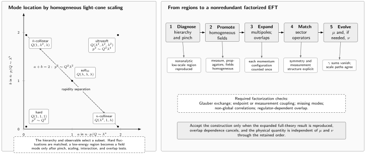
Collinear and soft-II modes lie on one virtuality line at different rapidities, ultrasoft lies at lower virtuality, and the construction adds multipole and overlap tests before factorized evolution. — Mode locations are shown in the exponents $a$ and $b$ of $(n\!\cdot p/Q,\bar n\!\cdot p/Q)\sim(\lambda^a,\lambda^b)$ , with the transverse exponent written in each label. The line $a+b=2$ contains $n$ -collinear, $\bar n$ -collinear, and soft-II scalings of virtuality $Q^2\lambda^2$ ; their separation along the line is a rapidity separation. Ultrasoft momentum has virtuality $Q^2\lambda^4$ , while hard fluctuations are matched at $Q^2$ . The points are alternatives selected by a hierarchy and observable, not a universal simultaneous field list. A consistent construction requires homogeneous fields, multipole and overlap expansion, sector matching, and $\mu$ and, when needed, $\nu$ evolution, with explicit factorization checks. The diagram is schematic and not to scale.

Regions, fields, matching steps, and scales

Four related objects should not be conflated.

Object	Definition	Acceptance evidence
Integration region	A homogeneous domain used to asymptotically expand an integral	Its expanded contribution is required for the target asymptotic series
EFT mode	A field representing a long-distance region across the declared low-energy problem	Homogeneous action, allowed interactions, reproduced infrared behavior, and controlled overlaps
Matching step	Removal of fluctuations not retained as dynamical modes	The full-minus-EFT difference is local at the retained order
Factorization scale	An auxiliary boundary used to separate renormalized sector contributions	Scale dependence cancels after coefficients, functions, and evolution are combined

The hard region in the Sudakov example is an integration region and a matching contribution, not a low-energy field. The two collinear and ultrasoft regions are integration regions and EFT modes. The scale $\mu_h\sim Q$ is chosen near hard matching, while lower natural scales are inferred from the mode virtualities. Later pages add overlap subtractions, operator matching, and evolution; this page does not assume factorization merely from the mode list.

Potential and ultrasoft modes beyond light-cone kinematics

Nonrelativistic systems show why virtuality alone does not classify a mode. Decompose a heavy momentum as

P^\mu=Mv^\mu+k^\mu.

Near threshold, a heavy particle has residual scaling

k^0\sim Mv^2, \qquad |\mathbf k|\sim Mv.

A potential gauge exchange can share $k^0\sim Mv^2$ and $|\mathbf k|\sim Mv$ , so it is off shell by order $M^2v^2$ and can become an instantaneous potential after appropriate matching. Ultrasoft radiation has

k^0\sim|\mathbf k|\sim Mv^2, \qquad k^2\sim M^2v^4,

and remains a propagating mode. Soft radiation with all components of order $Mv$ is another possible region. Which fields remain depends on whether each configuration is pinched, on shell, or already encoded in potentials and Wilson coefficients. The same words “soft” and “ultrasoft” therefore denote different component tuples in light-cone and nonrelativistic power countings.

A reproducible mode record

For every candidate mode, retain:

the hard scales, small parameters, external kinematics, measurement, and target power;
the ordered momentum components and their exact scaling exponents;
virtuality, rapidity, integration-measure, propagator, and field scaling;
allowed leading and subleading interactions, including symmetry transformations;
the regulator and natural $\mu$ and $\nu$ scales;
every pairwise and nested overlap subtraction;
the expanded full-theory region that the mode reproduces; and
one summed-integrand, amplitude, or observable benchmark plus named failure cases.

For the Sudakov fixture, the minimum record is the five-row table above, the definition $P^2\sim L^2\sim\lambda^2Q^2$ , the fact that soft-II and Glauber expansions are scaleless in the stated regulator, and the boxed asymptotic sum. A reproducible calculation uses the same record structure with $\delta=\Gamma/M$ rather than light-cone $\lambda$ counting.

Common pitfalls

Promoting every region to a field. The hard region belongs in matching coefficients, and some naively leading regions are scaleless or forbidden by interactions. Apply all relevance tests before enlarging the EFT.

Classifying modes by virtuality alone. Collinear and soft-II modes can have the same virtuality but parametrically different rapidities. Conversely, potential and radiation modes can require energy–momentum rather than light-cone coordinates.

Treating a scaleless integral as zero information. In dimensional regularization a scaleless integral can hide cancelling ultraviolet and infrared poles. State the origin of the zero and verify the pole assignment when it enters matching or overlap subtraction.

Importing a mode list between observables. Measurements, masses, recoil, spectators, and Glauber pinches can change which regions are leading. Repeat the relevance and overlap tests for the declared observable.

Exercises

Which of the $n$ -collinear, $\bar n$ -collinear, and soft-II scalings listed above have the same virtuality?

Solution

All three have $p^2\sim Q^2\lambda^2$ . Their light-cone component ratios—and therefore their rapidities—differ, which is why virtuality evolution alone may not separate them.
What evidence would demote a proposed mode to an overlap rather than an independent field?

Solution

If its expanded integrand and measurement are exactly a limiting zero-bin of an existing mode, and adding it creates double counting removed by the overlap subtraction, it is not independent field content.

References

Becher, Thomas, Alessandro Broggio, and Andrea Ferroglia. 2015. Introduction to Soft-Collinear Effective Theory. Lecture Notes in Physics 896. Cham: Springer. DOI. Open PDF.
Manohar, Aneesh V., and Iain W. Stewart. 2007. “The Zero-Bin and Mode Factorization in Quantum Field Theory.” Physical Review D 76 (7): 074002. DOI. Open PDF.